How to Build an Inventory Calculator

Managing inventories - especially the finances surrounding them - can pose serious challenges and create mountains of admin work. Custom inventory calculator apps are a powerful solution.

We might need to regularly perform calculations around stock changes, valuations, efficiency, warehouse utilization, or other KPIs.

The trouble is that these kinds of calculations are often deceptively complex - with many of the figures we need stored in different locations, in different formats. Drawing out the insights we need can be time-consuming and fraught with scope for error.

Today, we’re going to see how Budibase can be used to create professional internal tools for performing all kinds of inventory calculations - based on existing data sources.

By the end, you’ll have a clear working understanding of how to use our open-source, low-code platform to output custom solutions based on your own internal workflows.

But first, let’s think about a bit of background.

What is an inventory calculator

An inventory calculator is a relatively simple internal tool that performs a defined transformation on our inventory data and returns the result - based on user inputs.

So, this is made up of three elements:

• A data layer - where the information we need about our inventory is stored.
• A process layer - where we define the calculations that we want to perform on our inventory data.
• An interface layer - where users can set certain parameters for the calculation and interact with the results.

The calculations themselves could be just about anything - but the most common use cases concern changes in stock levels or values across a given time period - or beginning and ending valuations.

What’s most important is the relationship between the interface and process layers - where users can specify certain parameters each time a calculation is performed.

For instance, the date range of the subset of items they want to include.

You might also like our guide to web application development .

What are we building?

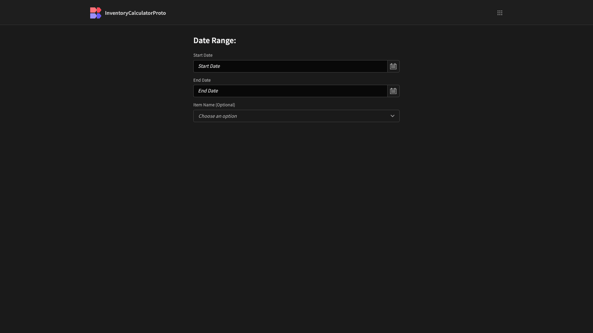
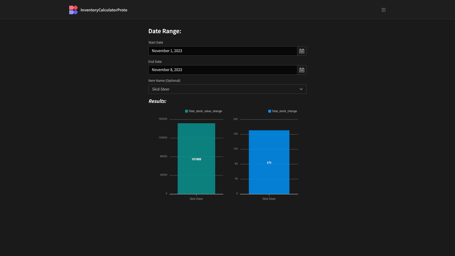
Our inventory calculator will be a simple form interface that enables users to calculate the net changes in their stock levels and values over a given time period. They can also specify whether they’d like to do this for specific items or on aggregate for the entire inventory.

Here’s what the completed form will look like:

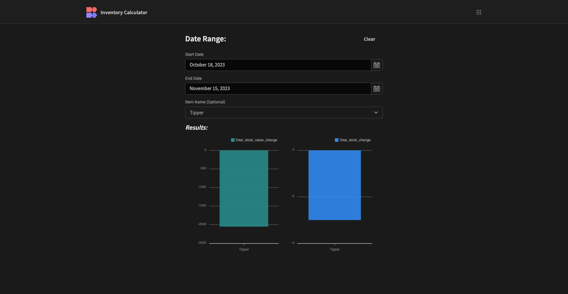
And here it is visualizing the results of our calculation:

Our calculator app is built around an existing PostgreSQL database, with tables storing information on our inventory, sales, returns, consignments, and shipments.

The logic for our calculations is contained in two custom queries. These accept bindable values to specify a date range and then calculate the net changes in our stock levels and values, based on the tables we just listed.

How to build an inventory calculator in 6 steps

So, let’s get started. If you haven’t already - sign up for a free Budibase account to start turning data into action.

1. Create a new Budibase application and connect your data

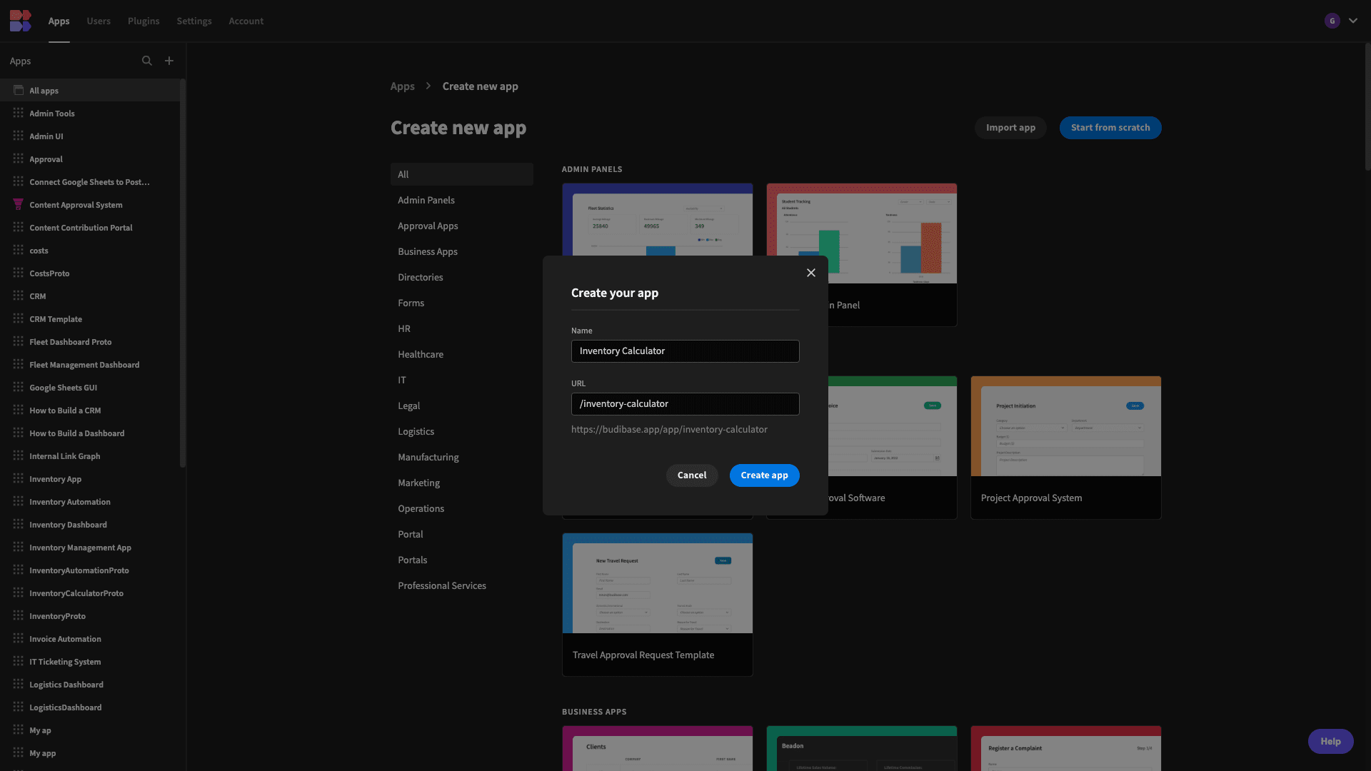
Our first step is to create a new Budibase application. We can start with a template or by importing an existing app - but today we’re starting from scratch. We can give our new app a name, which will also be used to generate a URL extension:

We then need to choose a data source for our app.

Budibase offers an internal database, as well as a huge range of dedicated connectors for SQL and NoSQL databases, alongside Google Sheets, REST API, and more.

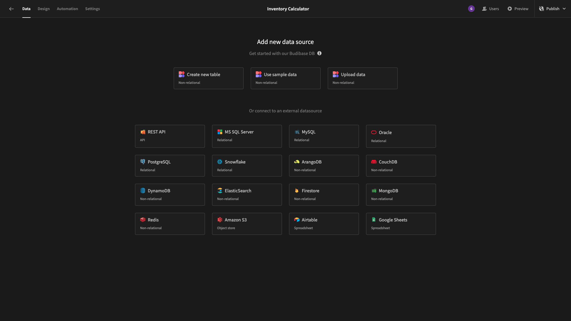
Again, we’re going to use Postgres. When we select this, we’re prompted to input our config details:

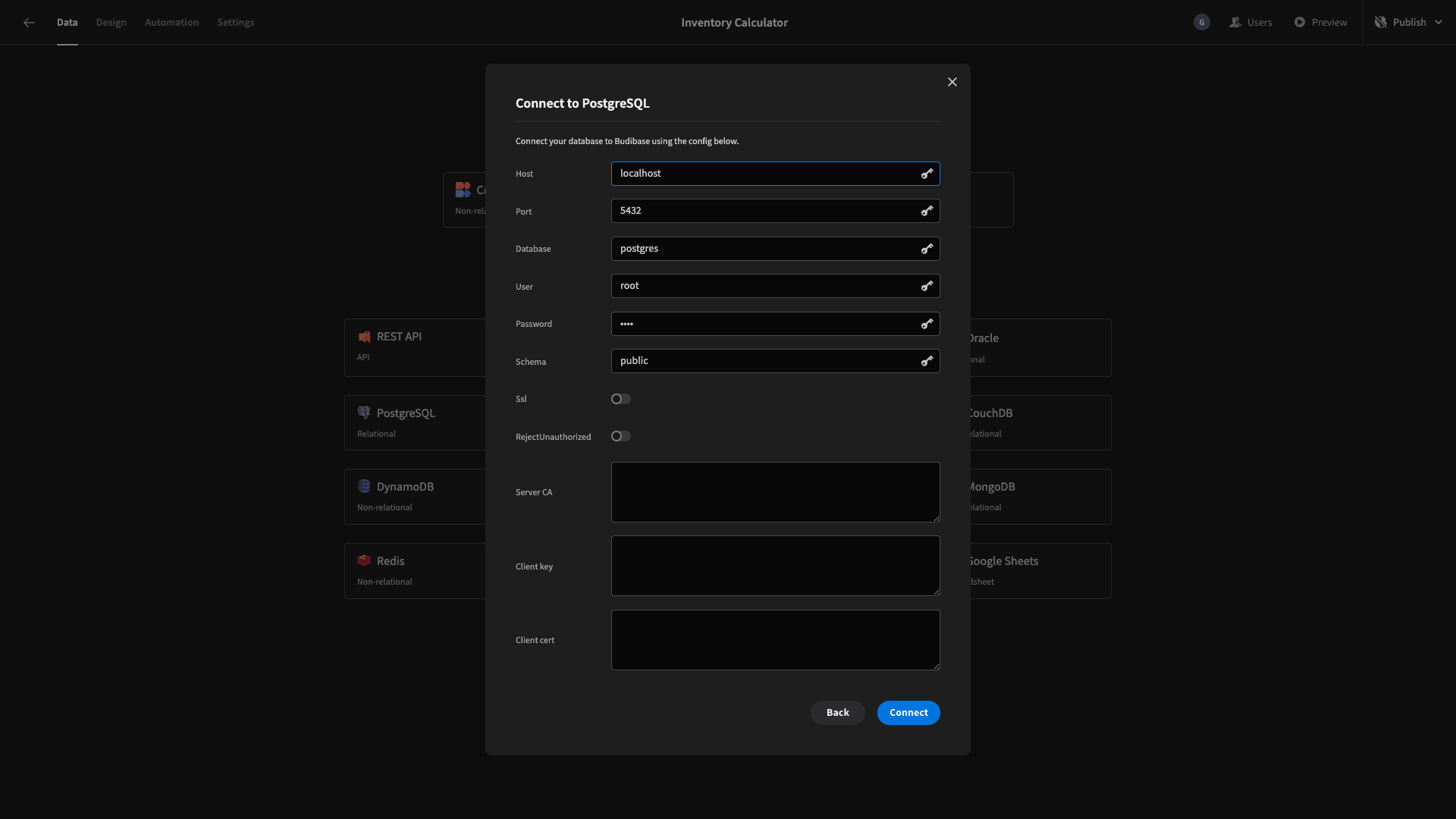
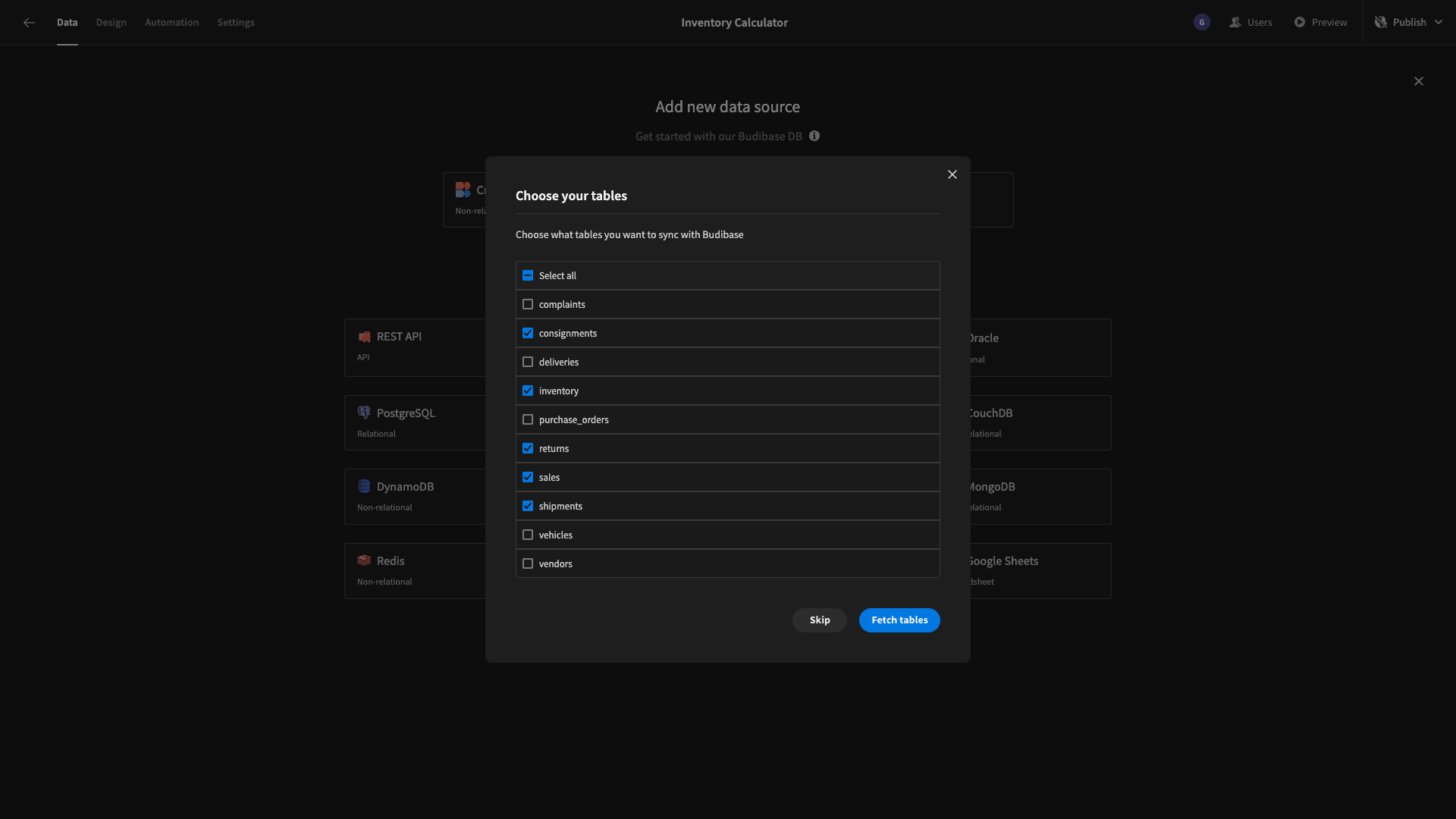
We can then choose which of our database’s tables we want to fetch so that they can be used and manipulated within Budibase. We can simply select them all - but we have tables we don’t need for this particular app project.

So, we’ll just select the five we listed earlier:

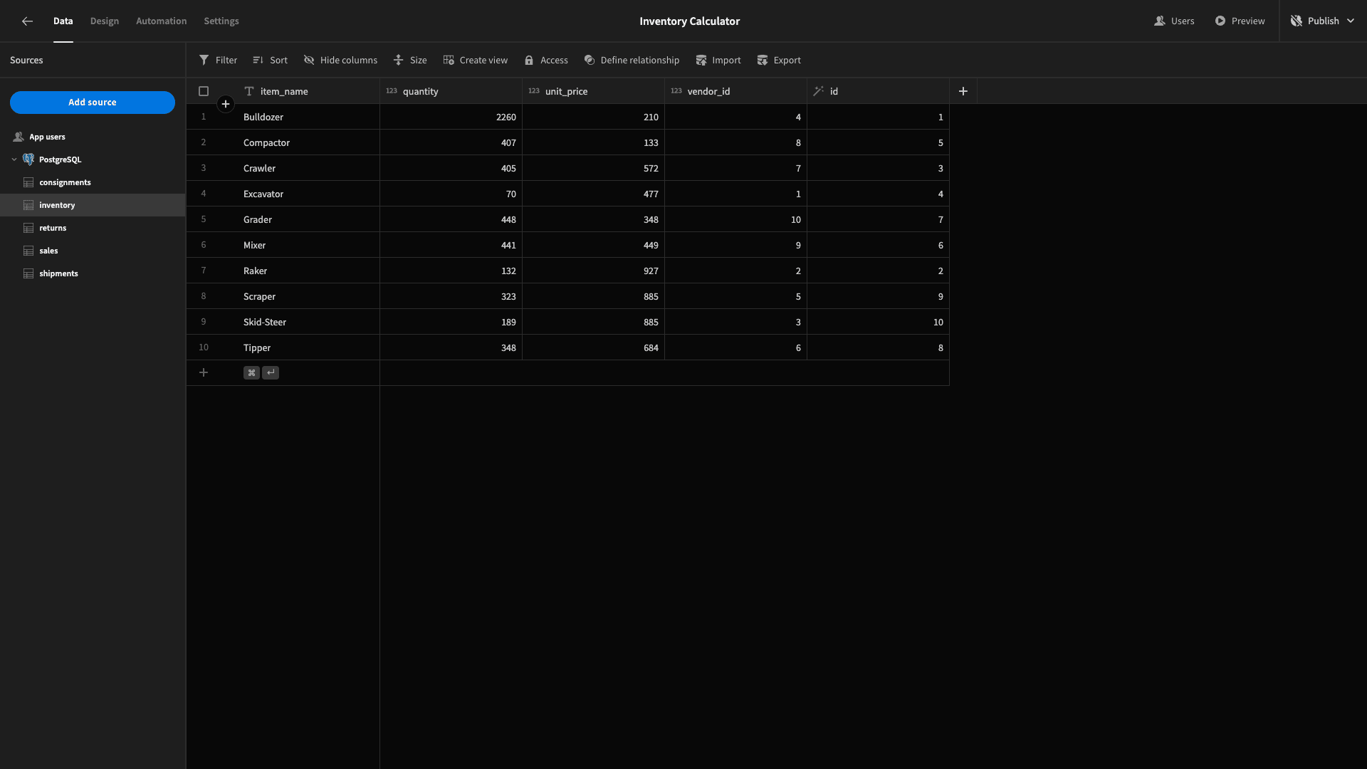
Straight away, we can perform CRUD operations in Budibase’s back-end - as well as editing the schema of our tables:

But, we’re going to build our inventory calculator’s logic around custom queries.

2. Writing our custom queries

Before we start writing queries for our inventory calculator - it’s worth taking a moment to understand our data model.

So, here’s a summary of what our five tables store and how they relate to one another.

• inventory represents the present state of our inventory, storing attributes called item_name, quantity, unit_cost, and a unique id.
• consignments represents our incoming stock, with an item_name, quantity, and consignment_number. Each entry links to rows in shipments and inventories with a shipment_id and inventory_id.
• shipments stores the purchase_date and arrive_date for each of the consignments entries related to it.
• sales stores an item_name, unique id, date, and quantity. It also links to the inventory table with an inventory_id attribute.
• returns stores a request_date, complete_date, reason, and a unique id. Each row also has a sale_id, relating to the original sales entry.

We need two queries. These will calculate the net change in stock - with sales entries reducing our inventory by a given quantity - and returns and consignments increasing our inventory for the stated quantity.

Our queries will also accept two bindable values that we’ll call startDate and endDate.

Let’s take a look at these one by one.

Head to your data source in Budibase and hit create new query.

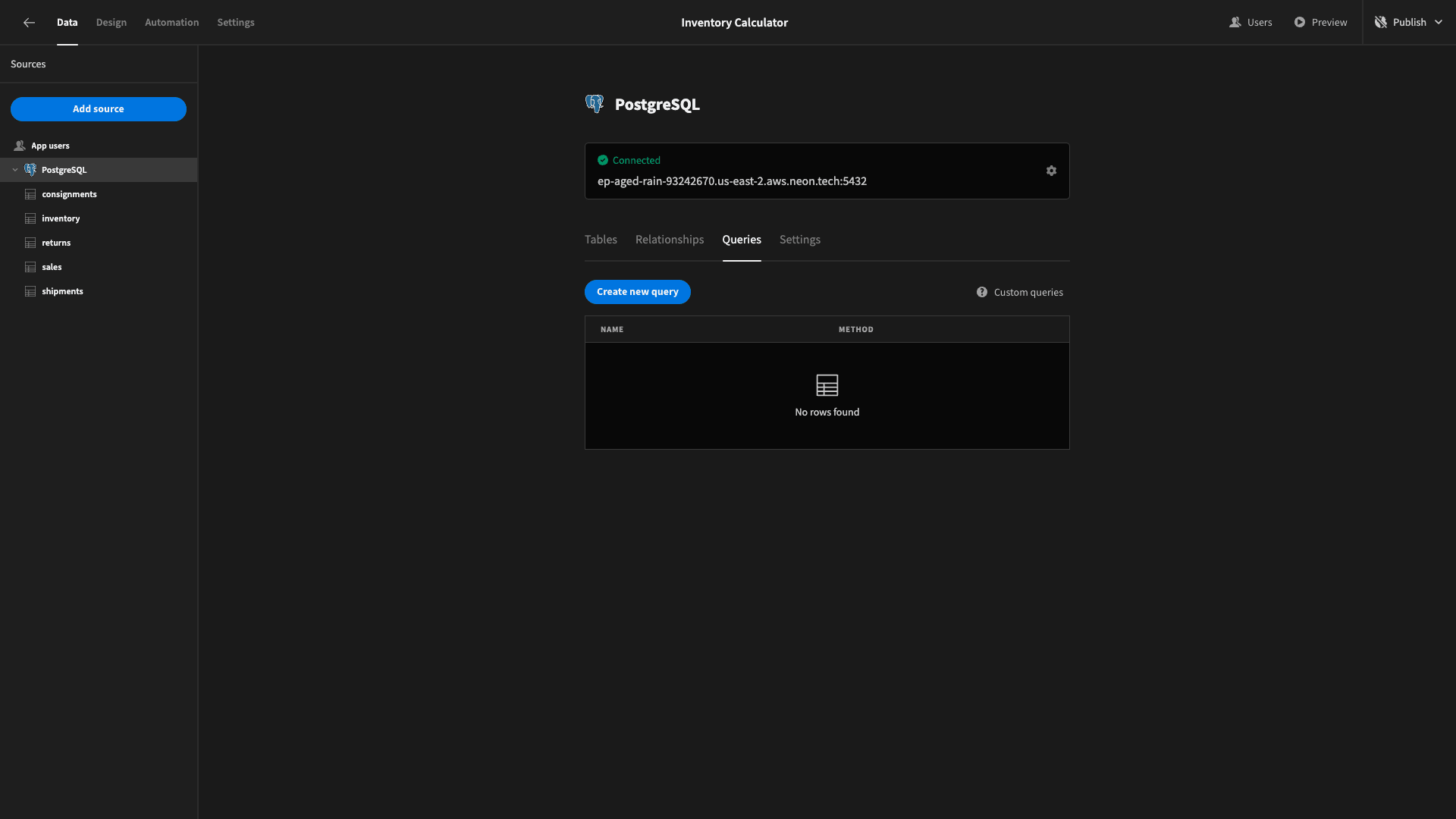
We’ll call the first one InventoryChangeByItem.

We want this to return the item_name, total_stock_change, and total_stock_value_change for each row in our inventory table in the given time frame.

The first thing we want to do is create our bindable values under the bindings heading. We can also give these default values - for the sake of testing our query, although we’ll eventually use user inputs to populate them:

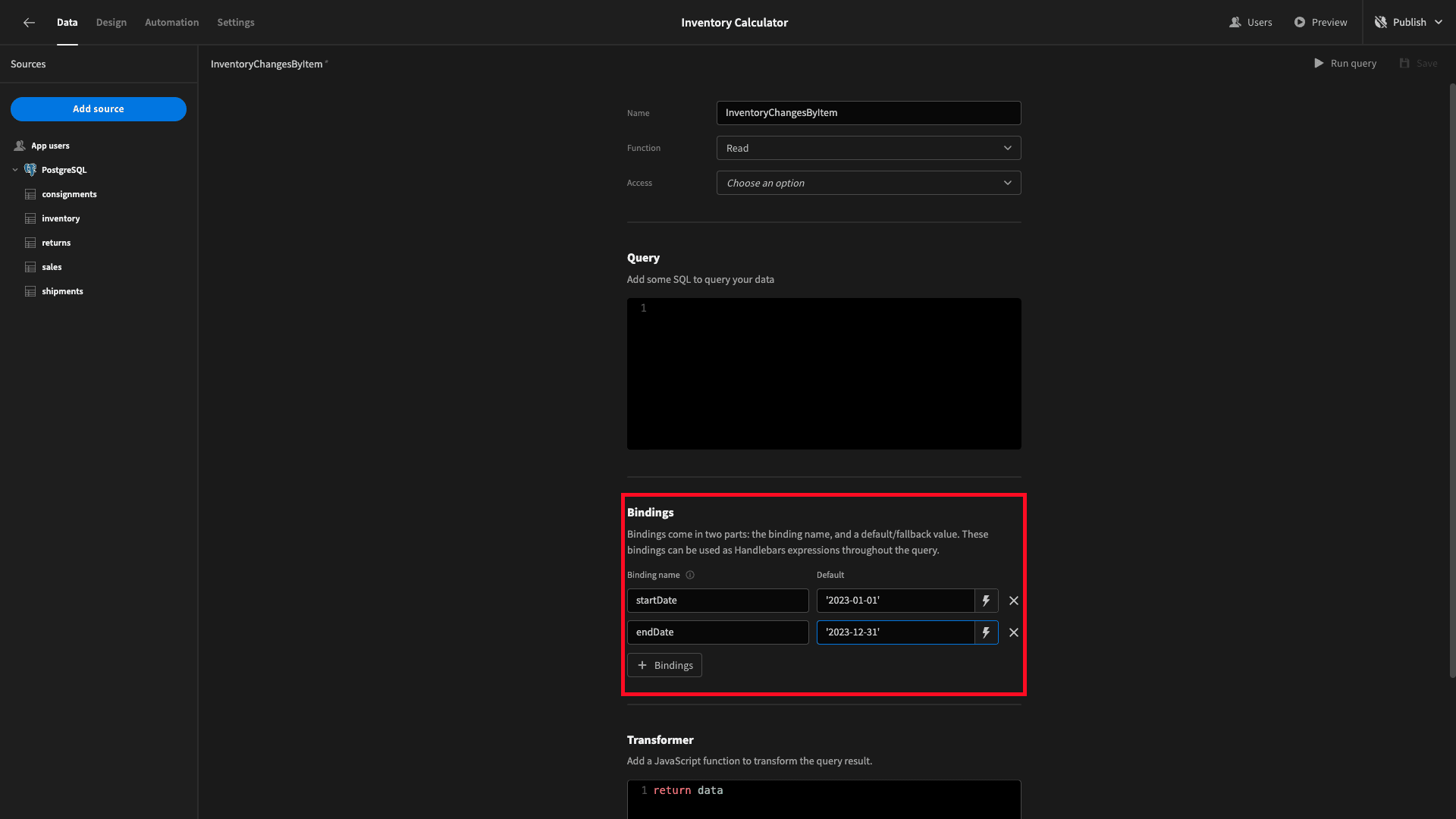
We can use these as handlebars expressions throughout our query.

Now, we’re ready to start writing the query itself. This will be relatively complex, so we’re going to take it one step at a time.

The first thing we need to do is create a common table expression which will SELECT our two date inputs:

1WITH date_range AS (
2
3  SELECT 
4​    {{ startDate }}::DATE AS start_date, 
5​    {{ endDate }}::DATE AS end_date
6),

Then, we use a second CTE called AllStockChanges to gather the relevant details from our sales, returns, shipments, and consignments tables, and calculate the net stock changes for all sales, returns, and consignments, grouped by item_name:

 1AllStockChanges AS (
 2  SELECT
 3​    c.item_name,
 4​    DATE_TRUNC('month', s.arrive_date) AS month_year,
 5​    SUM(c.quantity) AS stock_change
 6  FROM consignments c
 7  JOIN shipments s ON c.shipment_id = s.shipment_number
 8  GROUP BY c.item_name, month_year
 9  UNION ALL
10
11  SELECT
12​    s.item_name,
13​    DATE_TRUNC('month', s.date) AS month_year,
14​    -SUM(s.quantity) AS stock_change
15  FROM sales s
16  GROUP BY s.item_name, month_year
17  UNION ALL
18
19  SELECT
20​    s.item_name,
21​    DATE_TRUNC('month', r.complete_date) AS month_year,
22​    -SUM(s.quantity) AS stock_change
23  FROM sales s
24  JOIN returns r ON s.id = r.sale_id
25  GROUP BY s.item_name, month_year
26
27)

Our main query then SELECTs the:

• item_name from AllStockChanges.
• The SUM of stock_change from AllStockChanges.
• The SUM of stock_change from AllStockChanges multiplied by unit_cost from inventory.

We’ll also use two JOIN statements:

• Linking AllStockChanges to date_range BETWEEN the specified dates.
• Linking AllStockChanges to inventory on the respective item_names.

And finally, we’ll GROUP and ORDER BY item_name.

 1SELECT
 2  a.item_name,
 3  SUM(a.stock_change) AS total_stock_change,
 4  SUM(a.stock_change ` i.unit_price) AS total_stock_value_change
 5
 6FROM AllStockChanges a
 7JOIN date_range d ON DATE_TRUNC('month', a.month_year) BETWEEN d.start_date AND d.end_date
 8JOIN inventory i ON a.item_name = i.item_name
 9GROUP BY a.item_name
10ORDER BY a.item_name;

When we put all of this together, our full query is:

 1WITH date_range AS (
 2  SELECT 
 3​    {{ startDate }}::DATE AS start_date, 
 4​    {{ endDate }}::DATE AS end_date
 5),
 6
 7AllStockChanges AS (
 8  SELECT
 9​    c.item_name,
10​    DATE_TRUNC('month', s.arrive_date) AS month_year,
11​    SUM(c.quantity) AS stock_change
12  FROM consignments c
13  JOIN shipments s ON c.shipment_id = s.shipment_number
14  GROUP BY c.item_name, month_year
15  UNION ALL
16
17  SELECT
18​    s.item_name,
19​    DATE_TRUNC('month', s.date) AS month_year,
20​    -SUM(s.quantity) AS stock_change
21  FROM sales s
22  GROUP BY s.item_name, month_year
23  UNION ALL
24
25  SELECT
26​    s.item_name,
27​    DATE_TRUNC('month', r.complete_date) AS month_year,
28​    -SUM(s.quantity) AS stock_change
29  FROM sales s
30  JOIN returns r ON s.id = r.sale_id
31  GROUP BY s.item_name, month_year
32)
33
34SELECT
35  a.item_name,
36  SUM(a.stock_change) AS total_stock_change,
37  SUM(a.stock_change ` i.unit_price) AS total_stock_value_change
38FROM AllStockChanges a
39JOIN date_range d ON DATE_TRUNC('month', a.month_year) BETWEEN d.start_date AND d.end_date
40JOIN inventory i ON a.item_name = i.item_name
41GROUP BY a.item_name
42ORDER BY a.item_name;

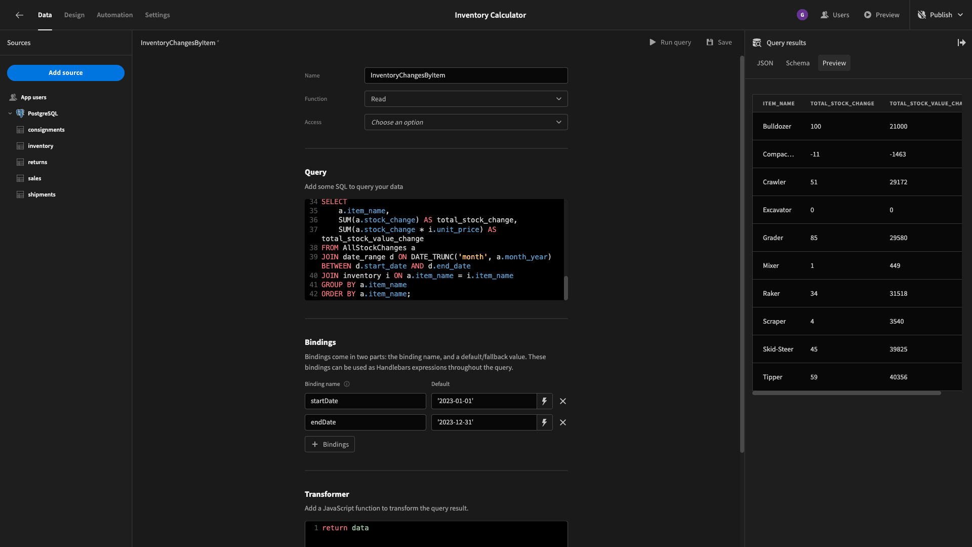
The data objects that are returned look like this:

1{
2 "item_name": "Bulldozer",
3 "total_stock_change": 100,
4 "total_stock_value_change": 21000
5}

We’ll save that and then duplicate it, so we don’t have to reconfigure our bindings for our second query.

We’ll call the new version InventoryChangesAggregate. This will also return the net stock and value changes from our inventory - but this time for the inventory as a whole, rather than broken up by item_name.

Our two CTEs will be exactly the same, but we need to make a couple of minor adjustments to our main query.

We’ll remove our GROUP BY and ORDER BY statements so that we just return a single data object for the entire inventory.

We also need to remove item_name from our SELECT statement. However, we still need a third attribute in our response. This is because want to place each of our two totals on separate bar graphs - so we need something to place on the Y axis of these.

So, we’ll add a string called totals and set it equal to ‘Total’.

Our new main query is:

1SELECT
2  'Total' AS totals,
3  SUM(a.stock_change) AS total_stock_change,
4  SUM(a.stock_change ` i.unit_price) AS total_stock_value_change
5FROM AllStockChanges a
6JOIN date_range d ON DATE_TRUNC('month', a.month_year) BETWEEN d.start_date AND d.end_date
7JOIN inventory i ON a.item_name = i.item_name;

And the full thing is:

 1WITH date_range AS (
 2
 3  SELECT 
 4​    {{ startDate }}::DATE AS start_date, 
 5​    {{ endDate }}::DATE AS end_date
 6),
 7
 8AllStockChanges AS (
 9
10  SELECT
11​    c.item_name,
12​    DATE_TRUNC('month', s.arrive_date) AS month_year,
13​    SUM(c.quantity) AS stock_change
14  FROM consignments c
15  JOIN shipments s ON c.shipment_id = s.shipment_number
16  GROUP BY c.item_name, month_year
17  UNION ALL
18
19  SELECT
20​    s.item_name,
21​    DATE_TRUNC('month', s.date) AS month_year,
22​    -SUM(s.quantity) AS stock_change
23  FROM sales s
24  GROUP BY s.item_name, month_year
25  UNION ALL
26
27  SELECT
28​    s.item_name,
29​    DATE_TRUNC('month', r.complete_date) AS month_year,
30​    -SUM(s.quantity) AS stock_change
31  FROM sales s
32  JOIN returns r ON s.id = r.sale_id
33  GROUP BY s.item_name, month_year
34)
35
36SELECT
37  'Total' AS totals,
38  SUM(a.stock_change) AS total_stock_change,
39  SUM(a.stock_change ` i.unit_price) AS total_stock_value_change
40FROM AllStockChanges a
41JOIN date_range d ON DATE_TRUNC('month', a.month_year) BETWEEN d.start_date AND d.end_date
42JOIN inventory i ON a.item_name = i.item_name;

The response looks like this:

1{
2 "totals": "Total",
3 "total_stock_change": 368,
4 "total_stock_value_change": 193977
5}

Now, we’ve got all of the data we need.

3. Building our input form

Our next step is to build an interface where users can set parameters and trigger our inventory calculator.

We’ll start by creating a new blank screen.

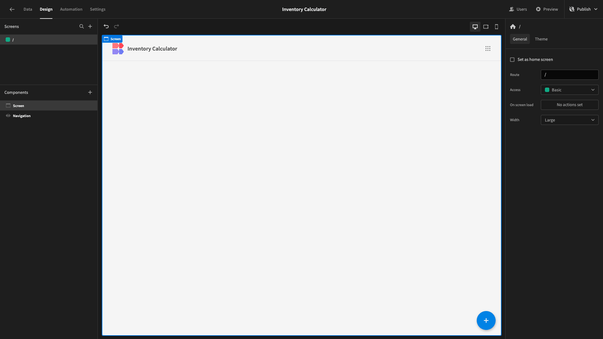
Eventually, this will contain two things:

1. A form that allows users to configure our calculation, by setting a date range and - optionally - a specific item.
2. A series of charts to visualize the results.

We’re going to start by adding a form component, which the rest of our form will be nested inside:

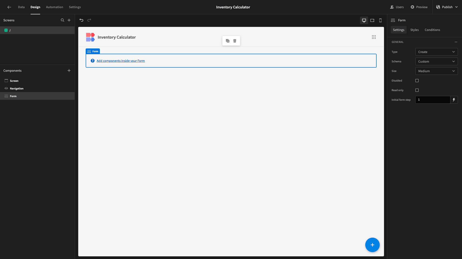
We can keep all of the default settings as they are.

Inside this, we’ll nest a container and set its horizontal alignment to center:

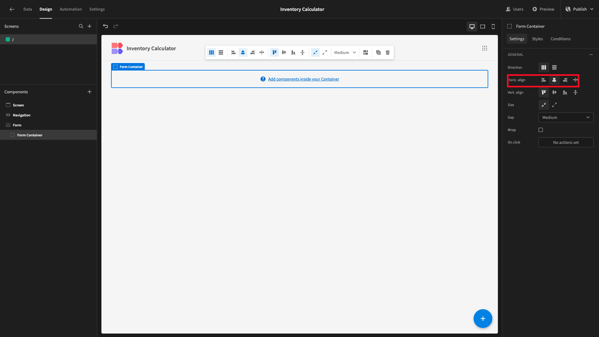
The first display elements we want are a headline that reads Date Range: and a button that will enable users to clear the form.

Start by adding a second container, this time setting its direction to horizontal. This time, we’ll leave the alignment as it is:

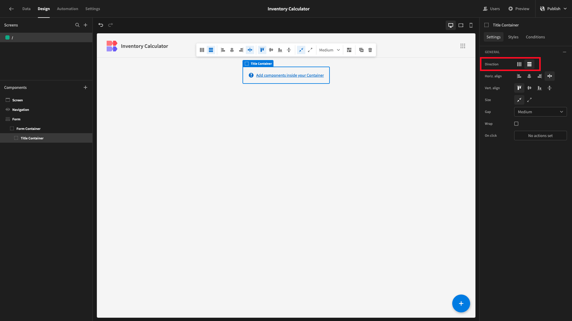
We’ll also give this a width of 50% under styles:

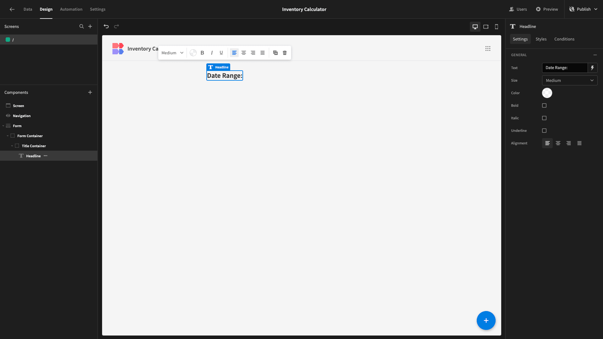
We’ll add a headline and set its text to Date Range:

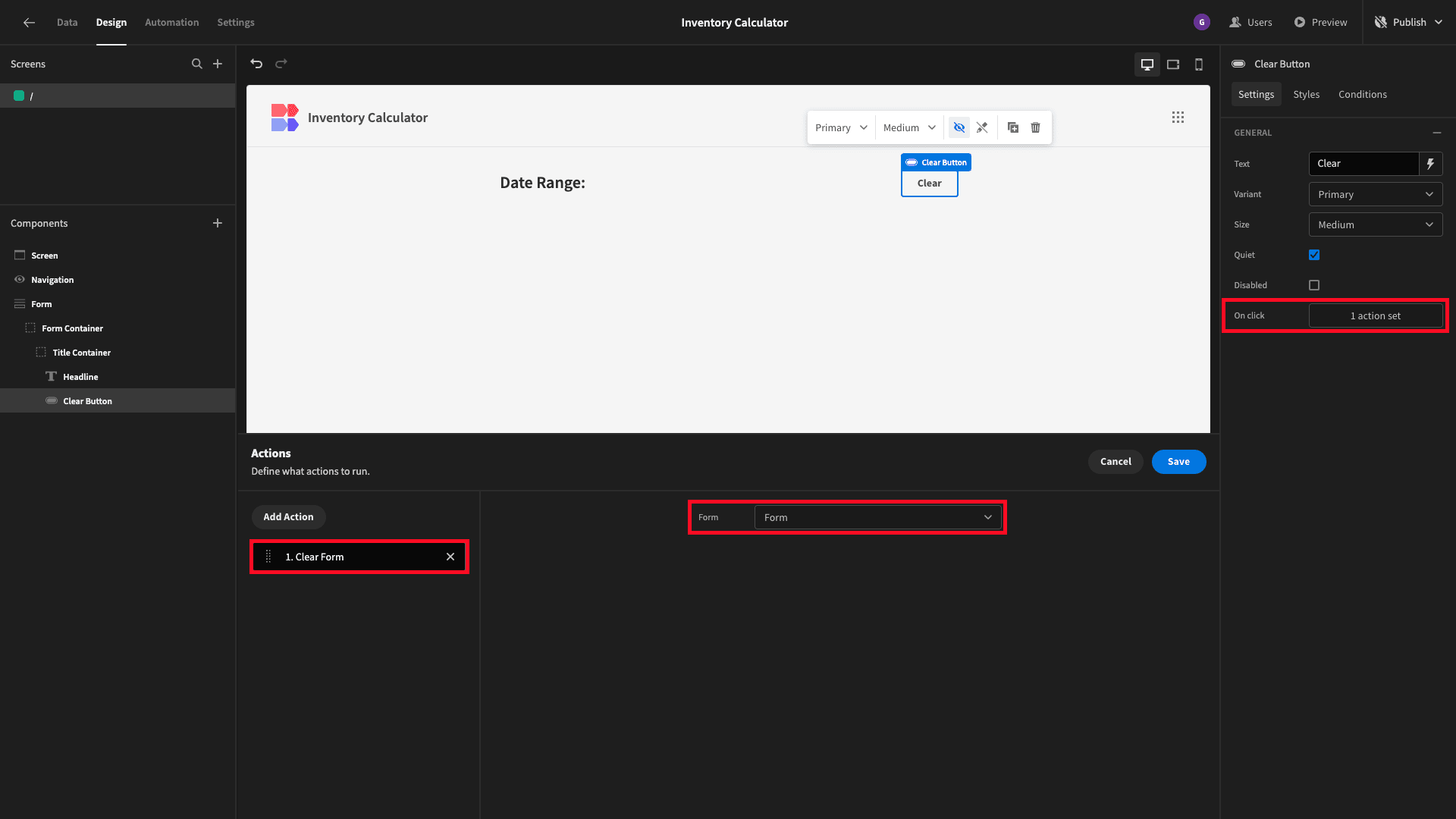
Beside this, we’ll place a button. We’ll check the quiet box and set the text to Clear:

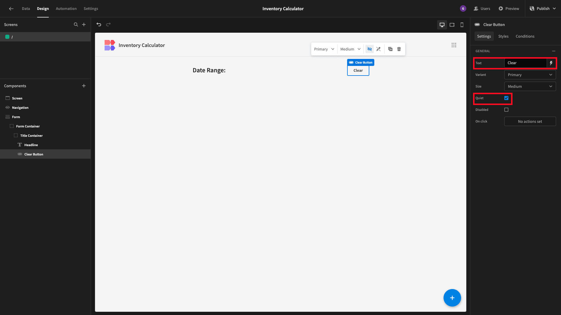
Lastly, under On-Click actions, we’ll add a clear form action - and point it at our form:

Of course, this won’t do anything until we build out our form a little more.

Beneath our second container, we’re going to add a field group:

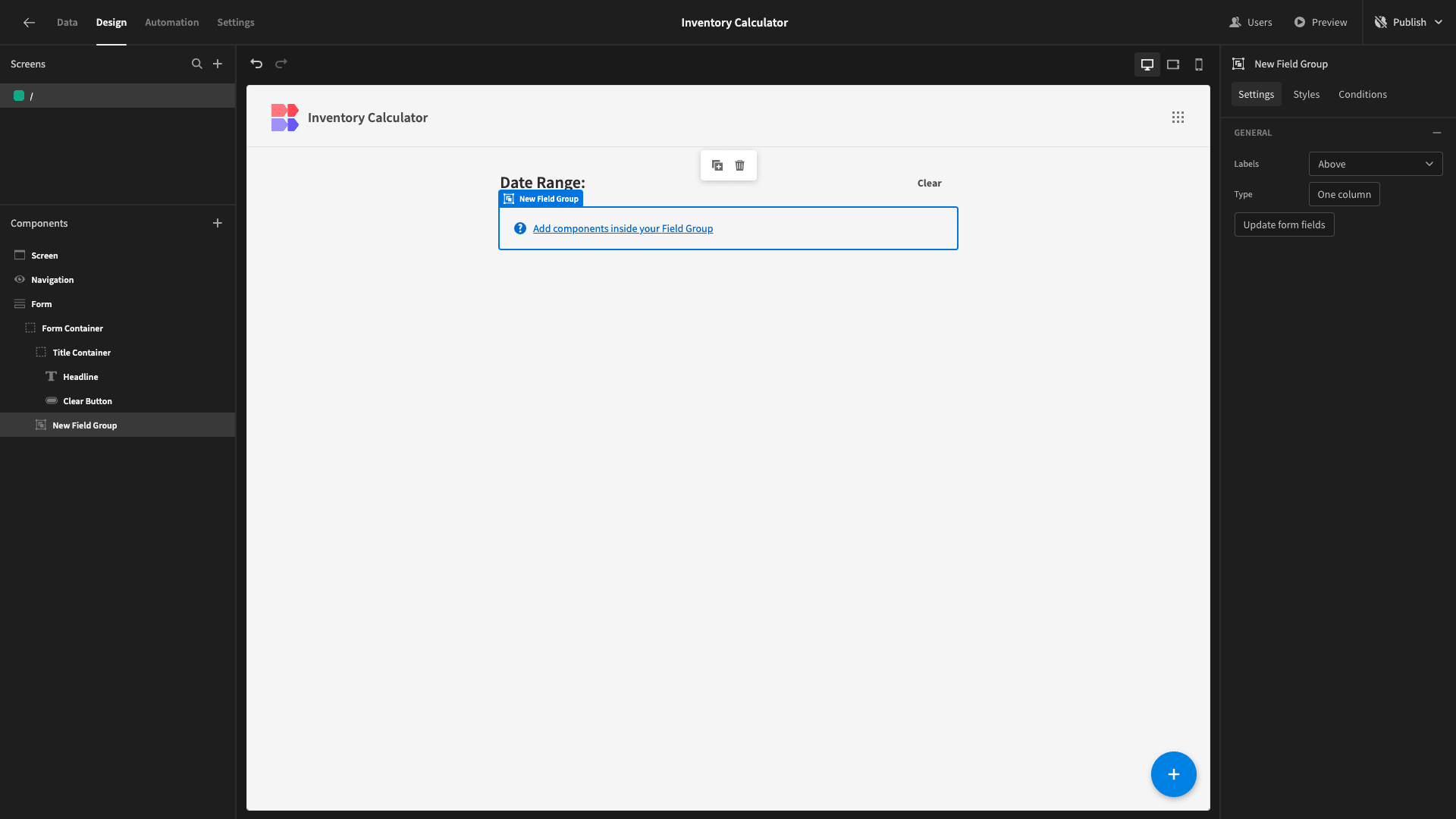
We’ll also set the width of this to 50%.

Inside this, we’re going to place the specific form fields that will allow users to configure our inventory calculator’s parameters.

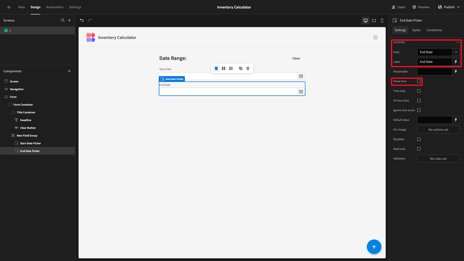
First of all, we’ll add two date pickers. On the first, we’ll set the field and label to Start Date. On the second, we’ll set these to End Date.

We’ll also deselect show time on both:

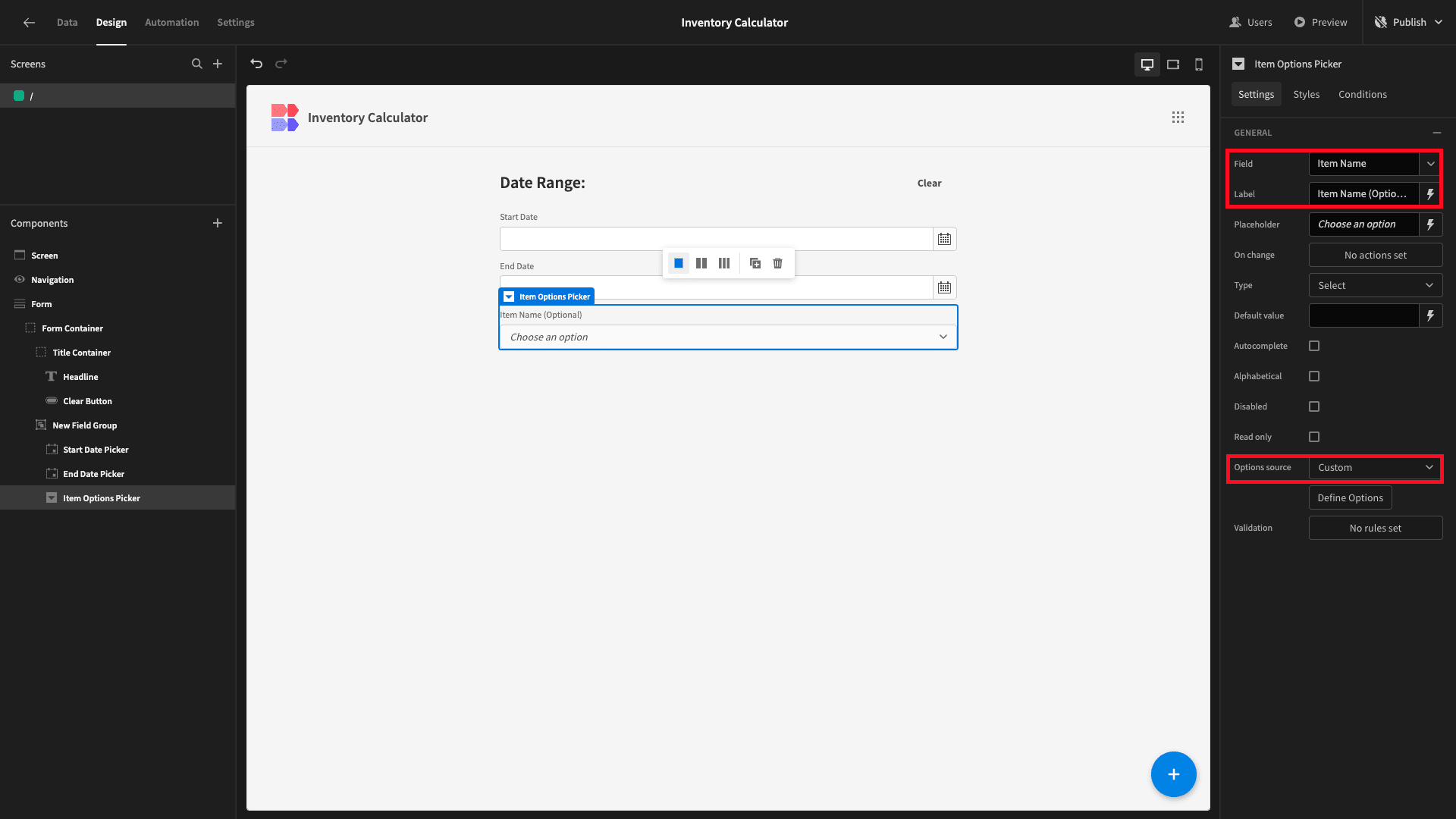
Beneath this, we’ll add an options picker. We can set the field to Item Name, the label to Item Name (Optional), and the options source to custom:

Then, we’ll hit define options - and input each of the possible item_names from our inventory table as labels and values:

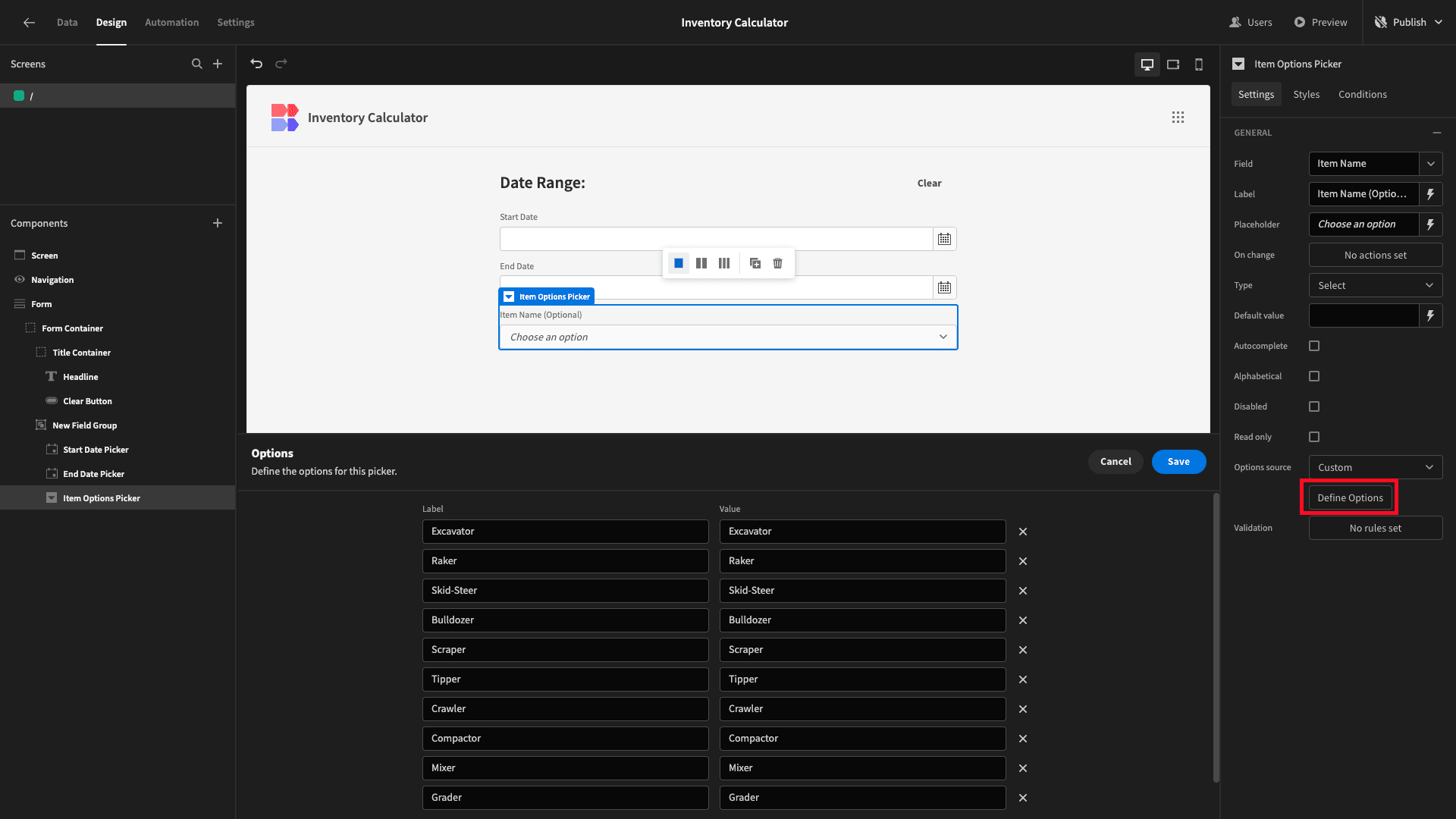
Here’s what our form looks like so far:

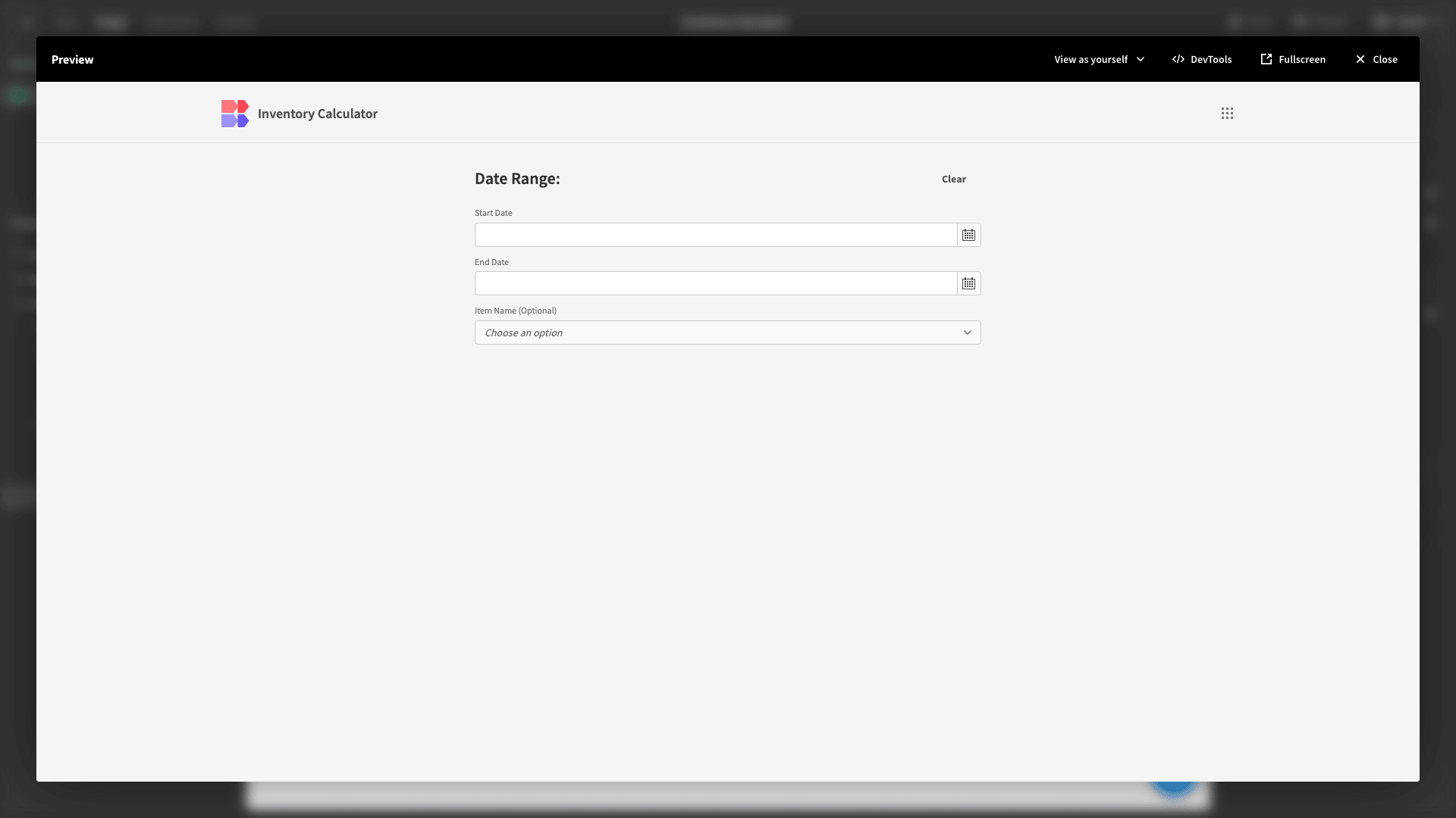
4. Building our results charts

Next, we want to create the bar charts that will display the results of our inventory calculations, based on the information that users have provided.

We’ll actually have two separate pairs of charts and display either one depending on whether or not the user has specified a particular item.

We’ll start by adding another horizontal container at the bottom of our original form container and setting the width to 50%:

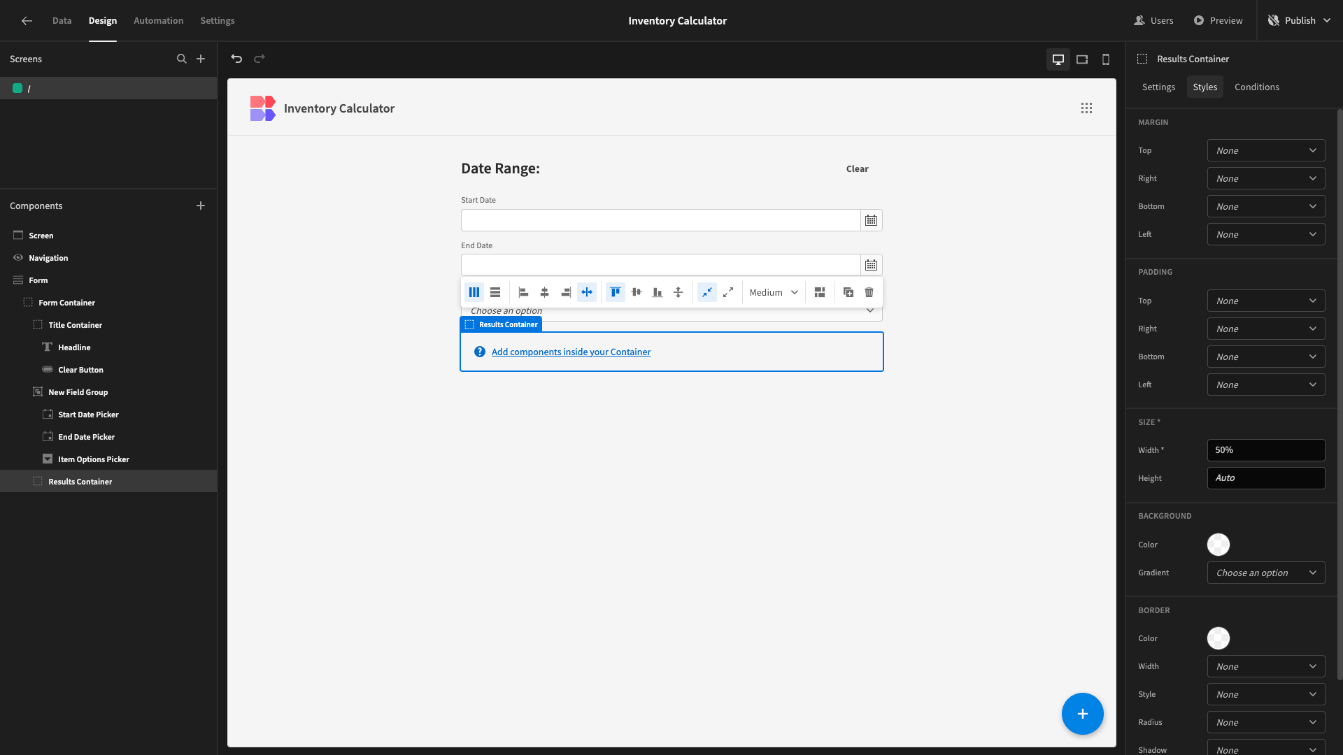
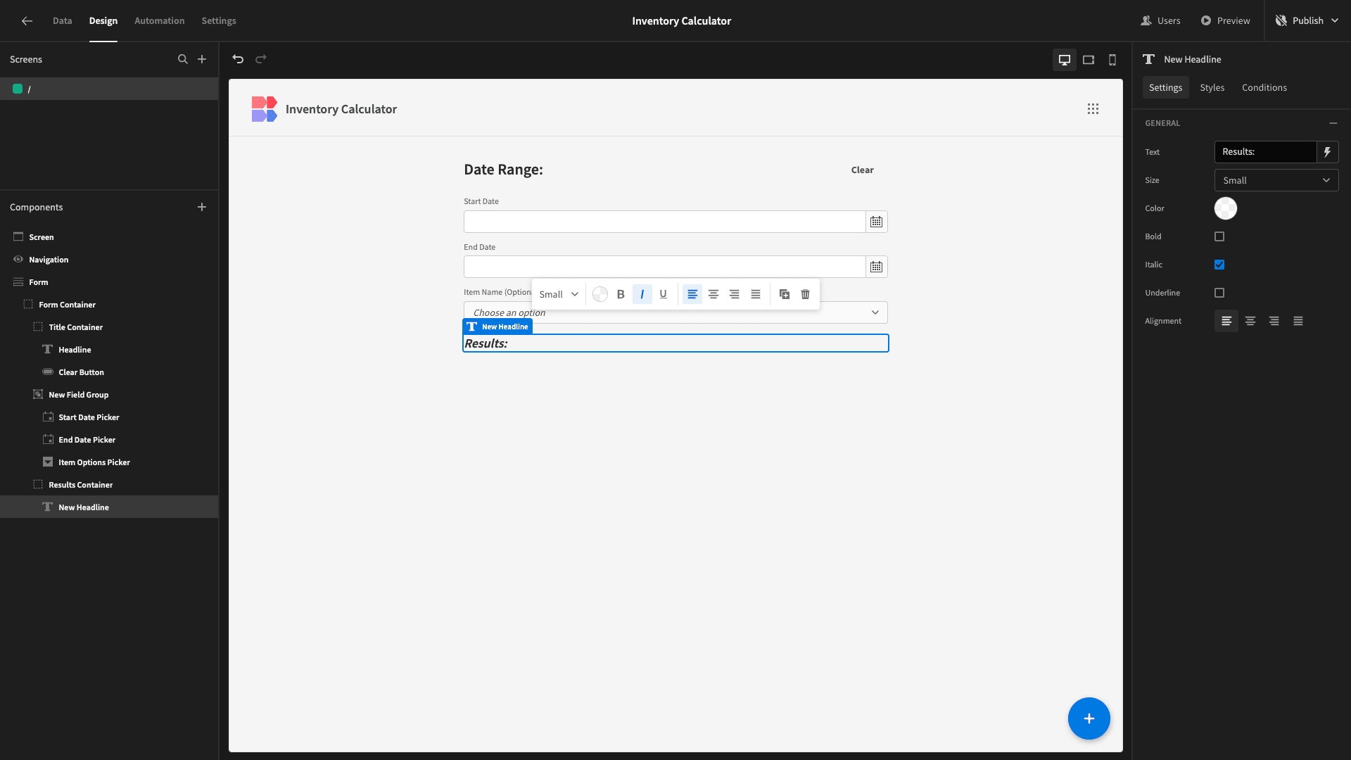
Inside this, we’ll place another headline, with its size set to small and its text to Results. We’ll also select the italic option:

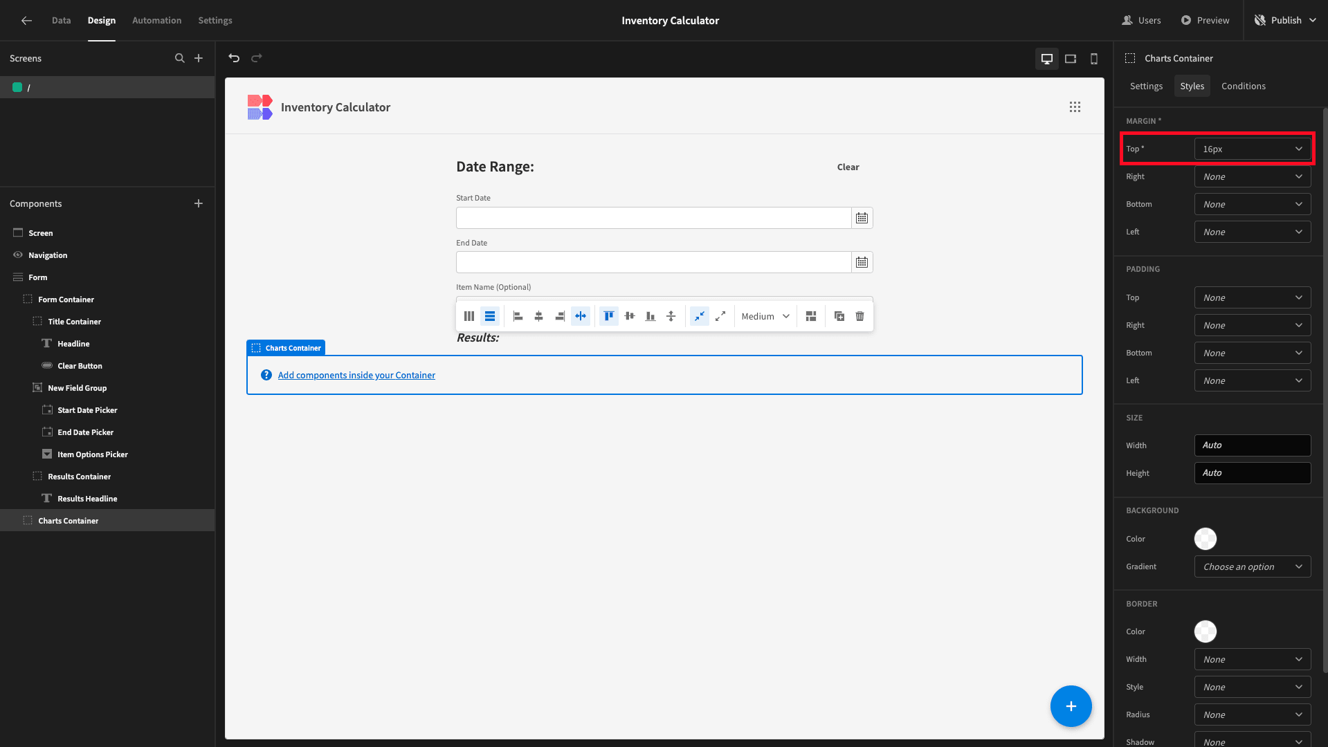
Beneath the form container, we’ll add another horizontal container. We’ll also give this 16px of padding to the top and set its alignment to center:

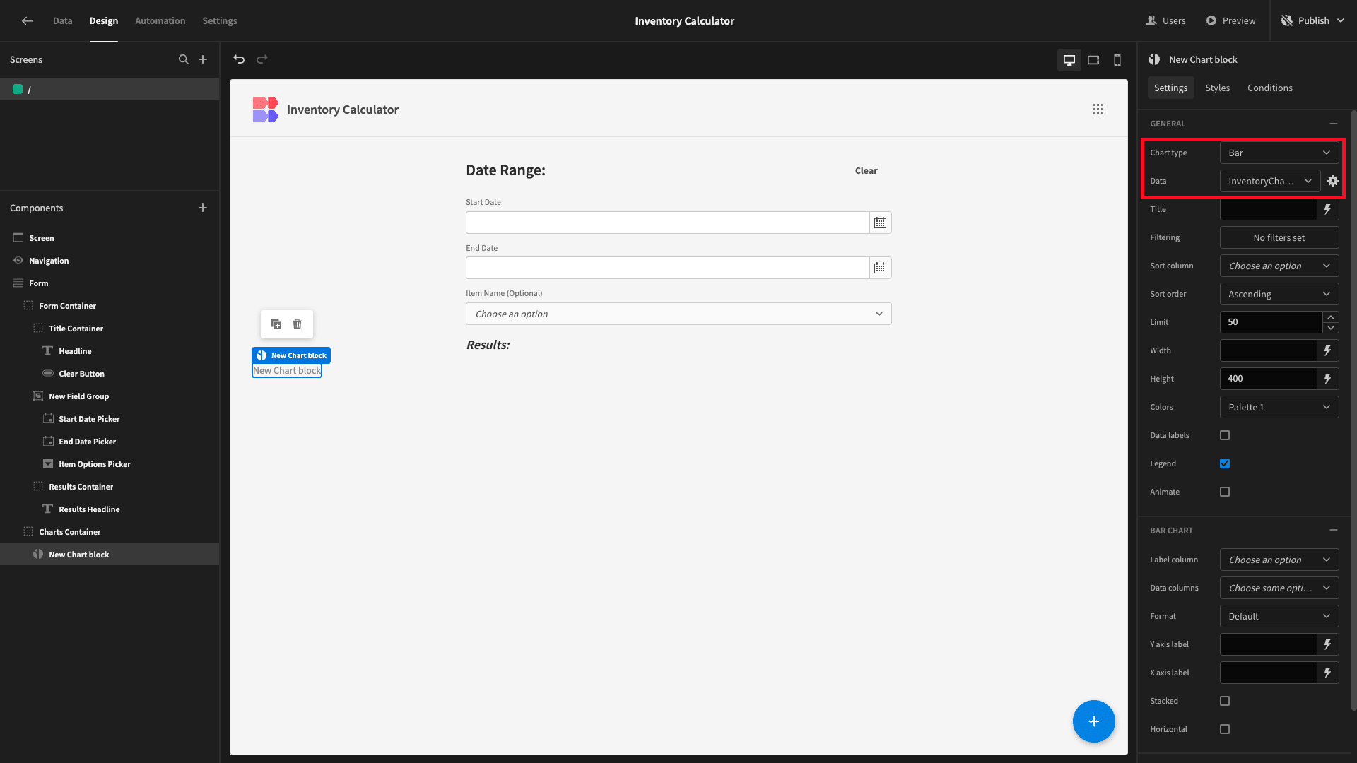
Inside this, we’ll add a chart block. We’ll set its type to bar and its data to our InventoryChangesAggregate query.

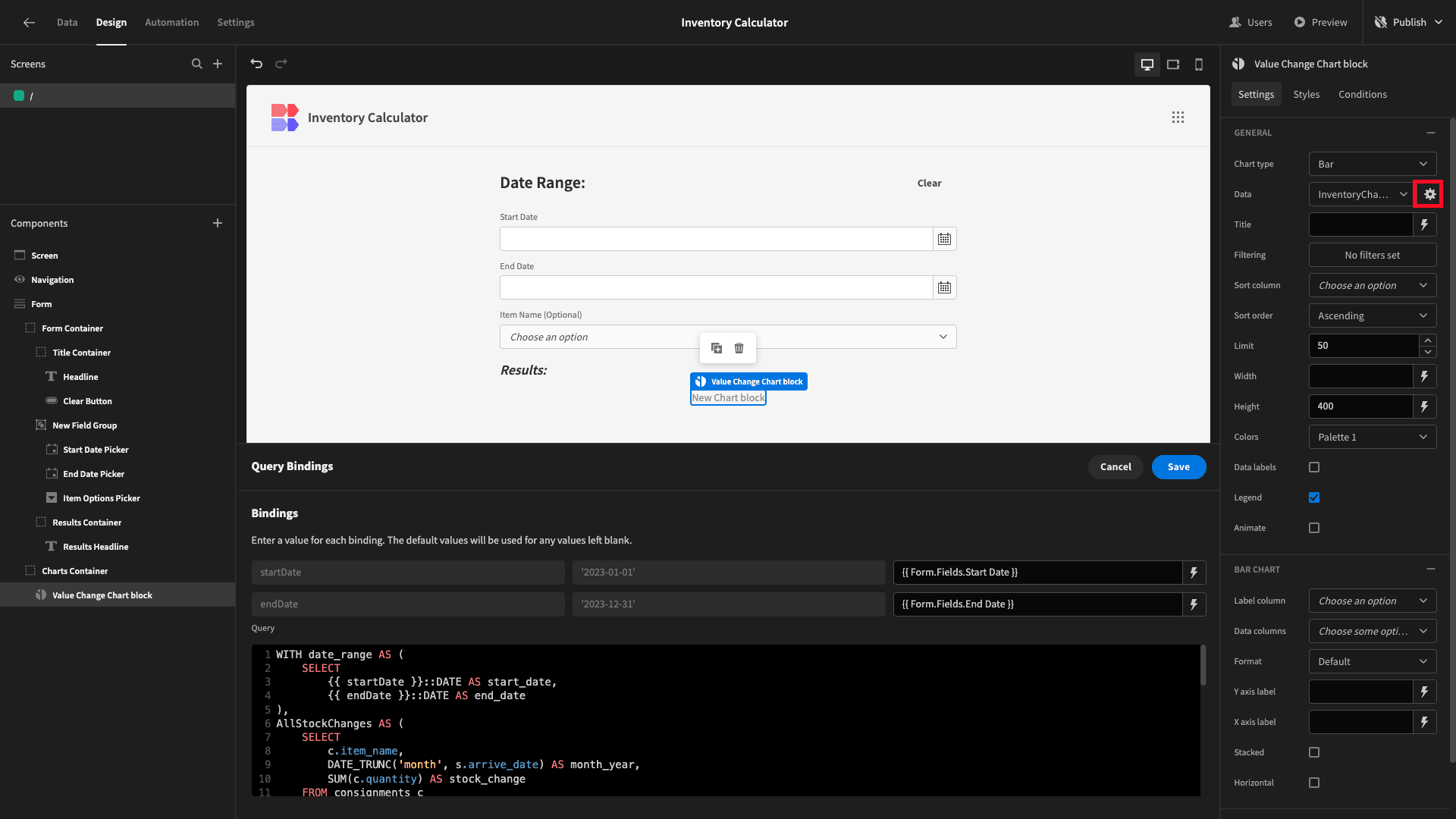
We’ll then open the settings for our data source, and bind the date parameters for our query to the outputs of our two date pickers, using {{ Form.Fields.Start Date }} and {{ Form.Fields.End Date }}.

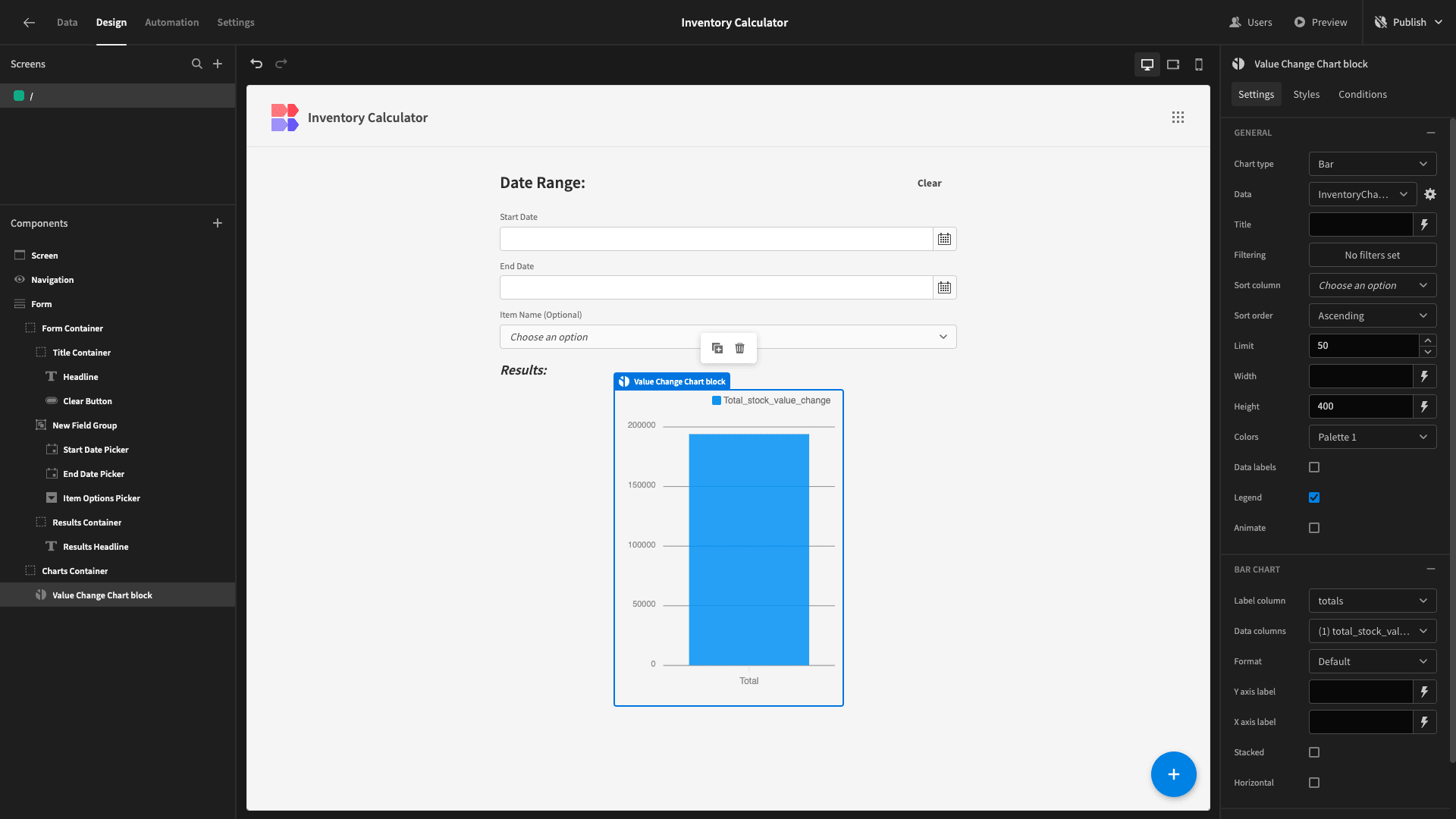
And lastly, we’ll set the label column to totals and the data column to total_stock_value_change.

Next, we’ll duplicate this chart - this time, swapping the data column for total_stock_change.

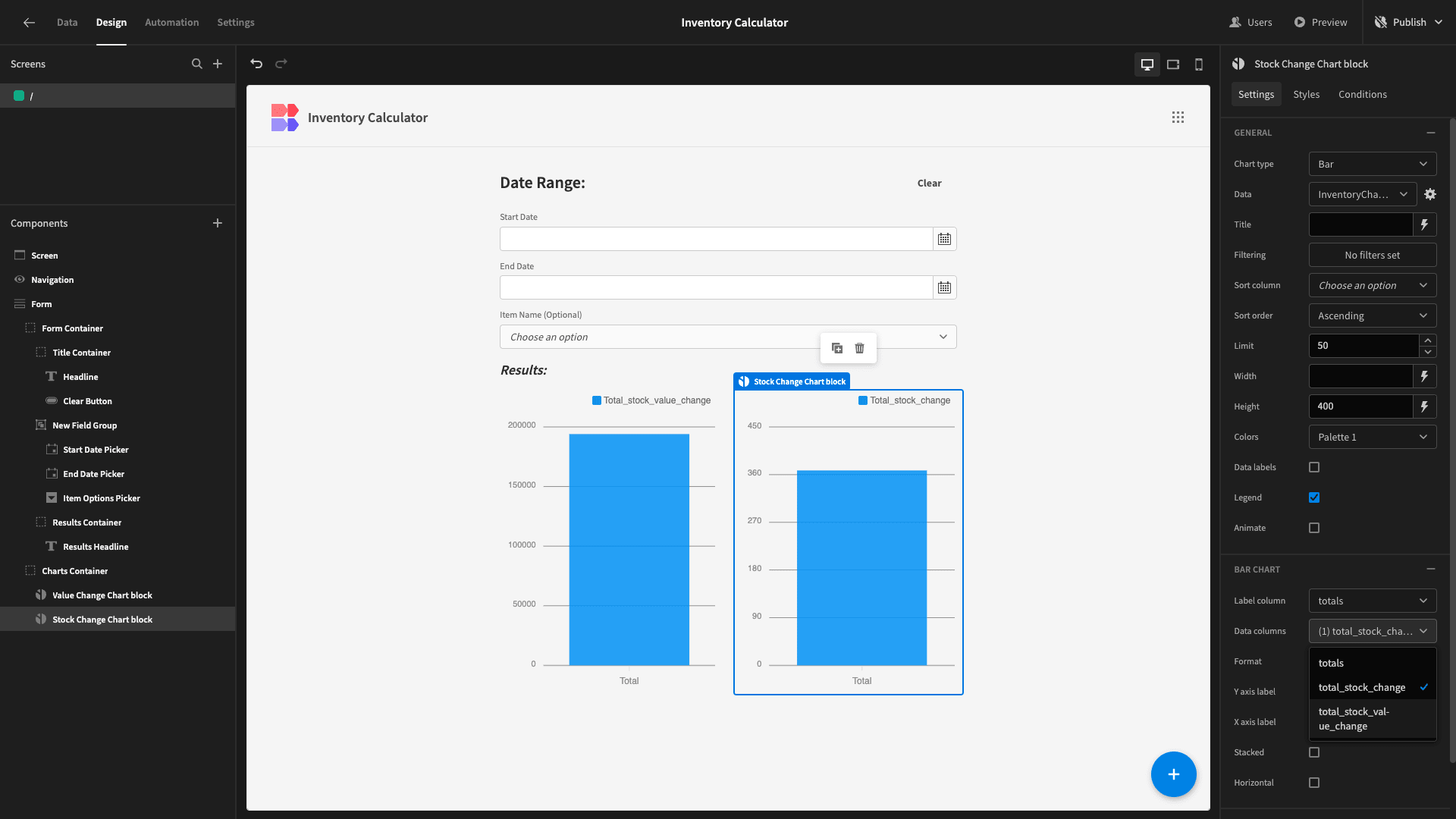
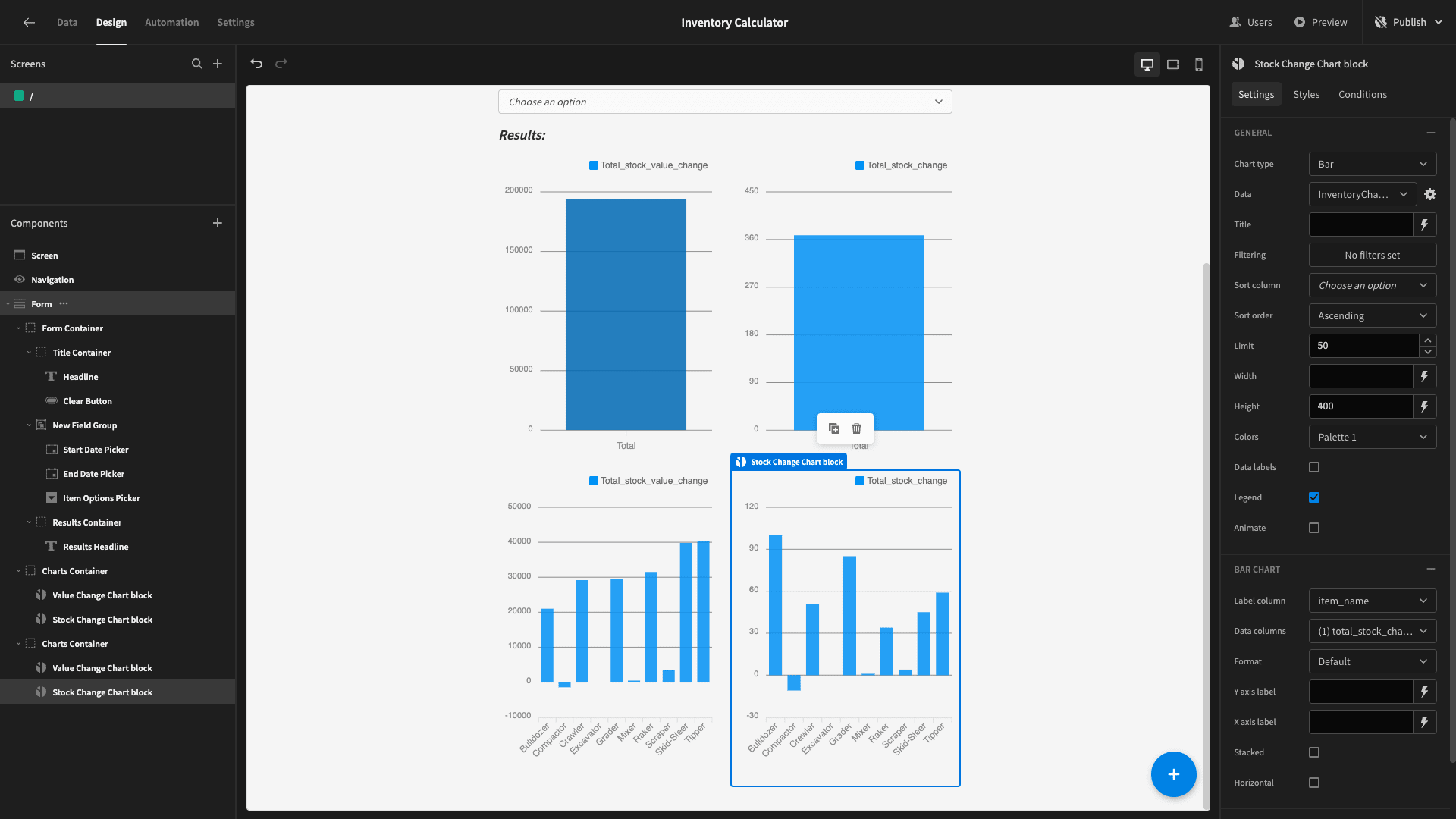
Then, we can duplicate the entire parent container, and change the new versions of our charts to point at InventoryChangeByItem query.

We’ll swap the label column to item_name, as well as remembering to configure our query bindings again:

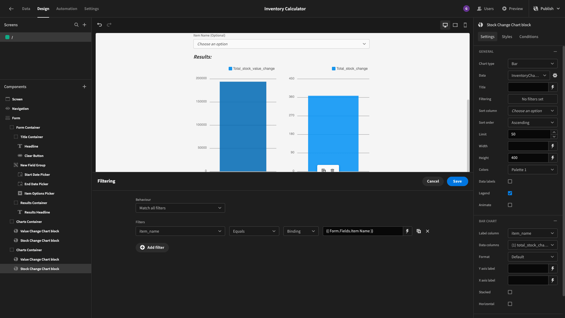
For one final step, we’ll also add filters to each of these charts, so that they only display the particular item that users have specified, by binding their item_name to {{ Form.Fields.Item Name }}.

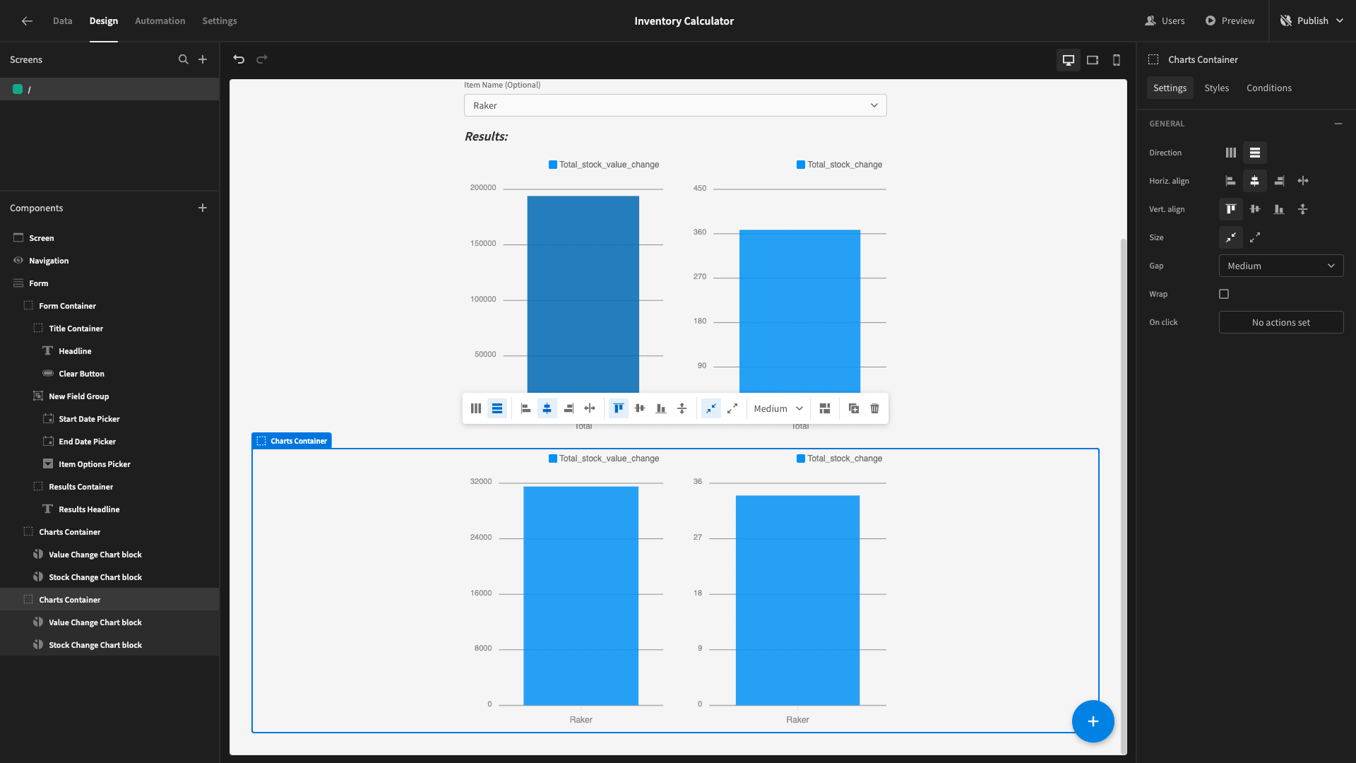
Here’s what this should look like:

5. Adding conditionality

Now, we only ever want to display two charts - not four. We’ll achieve this by applying conditionality rules to hide or display different elements, based on which form fields users have populated.

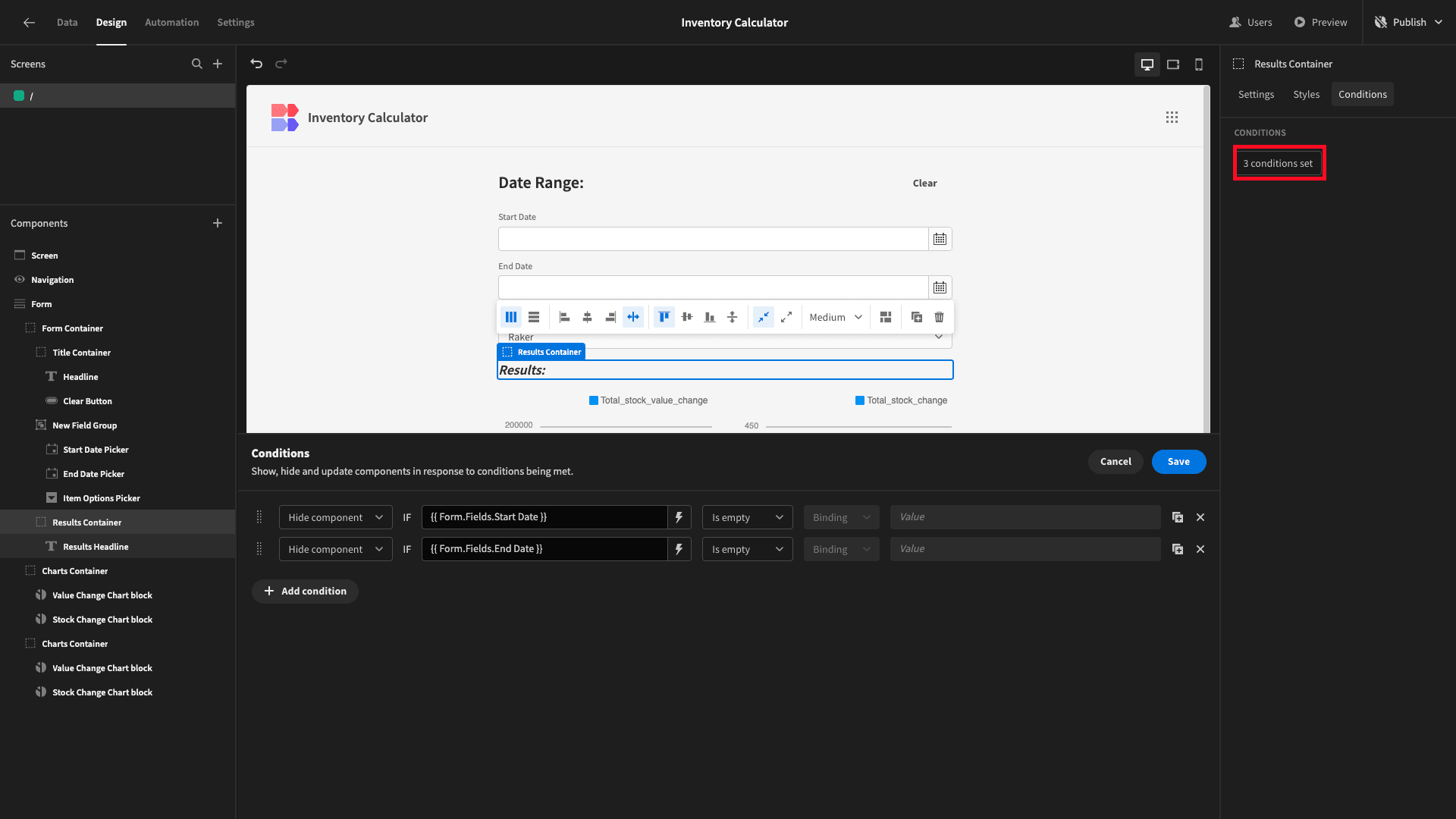
For the results container, we’ll add two rules, so that it’s hidden if either of our date pickers is empty:

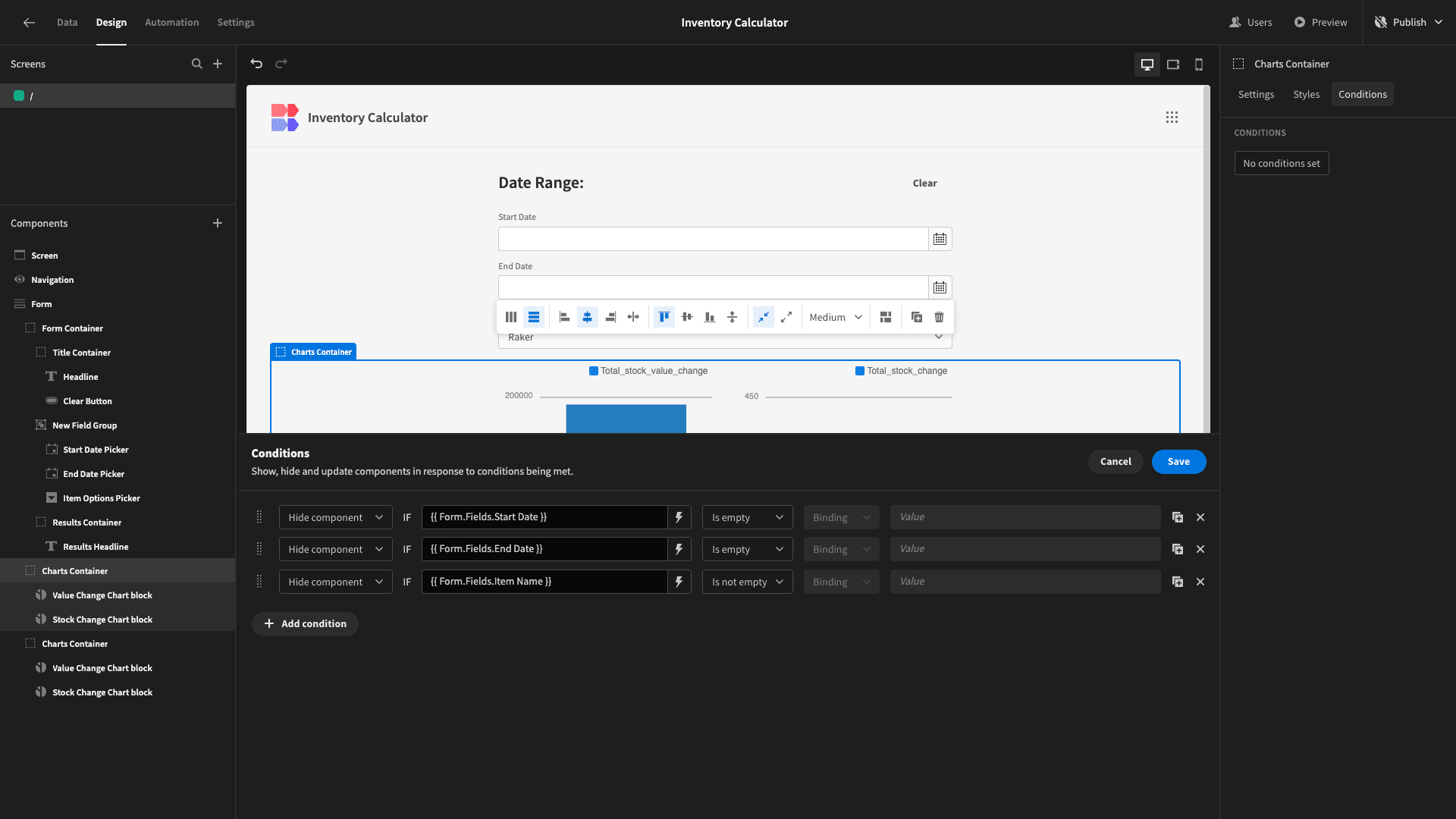
For our first charts container, we’ll set rules to hide it if the date pickers are empty and if the item name field is not empty:

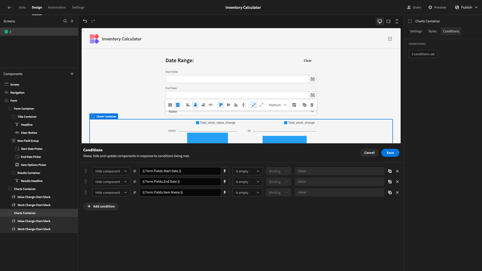
And finally, we’ll set the second chart container to be hidden if all three fields are empty:

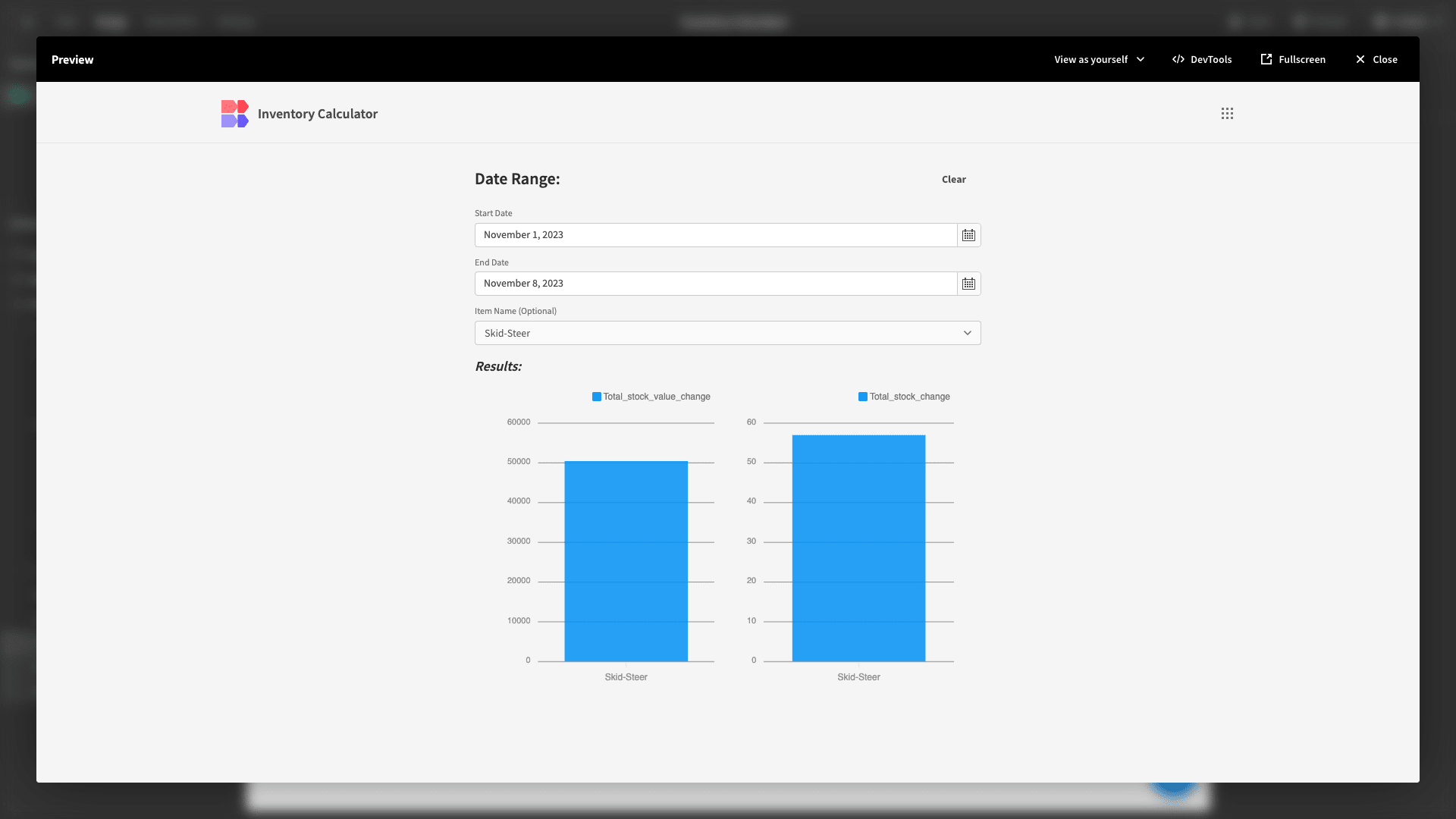
Here’s what we have so far:

6. Design tweaks and publishing

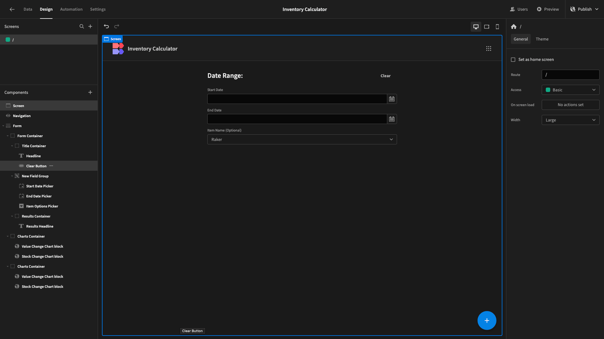
Before we publish our app, we’ll make a few UX improvements. First of all, we’ll hit screen and choose darkest under theme.

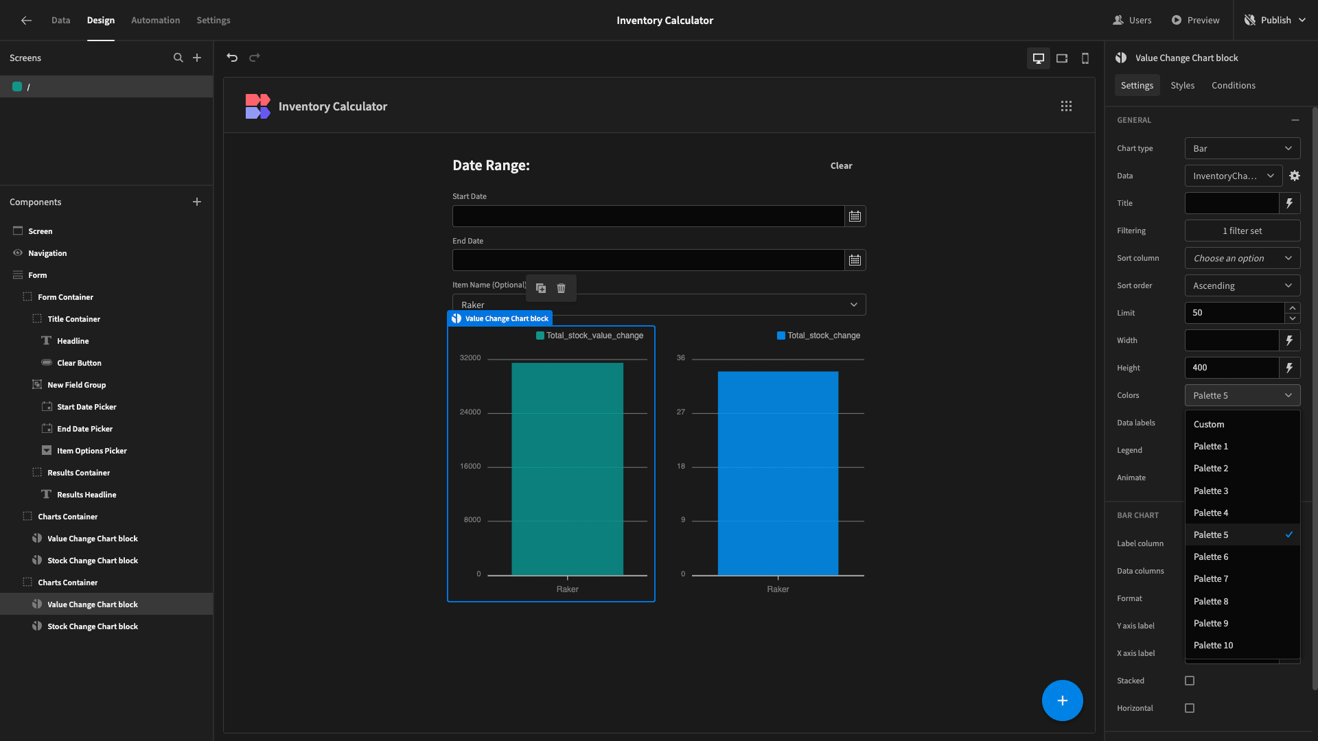
Then, we’ll play around with the color palettes of our charts, for better visual separation:

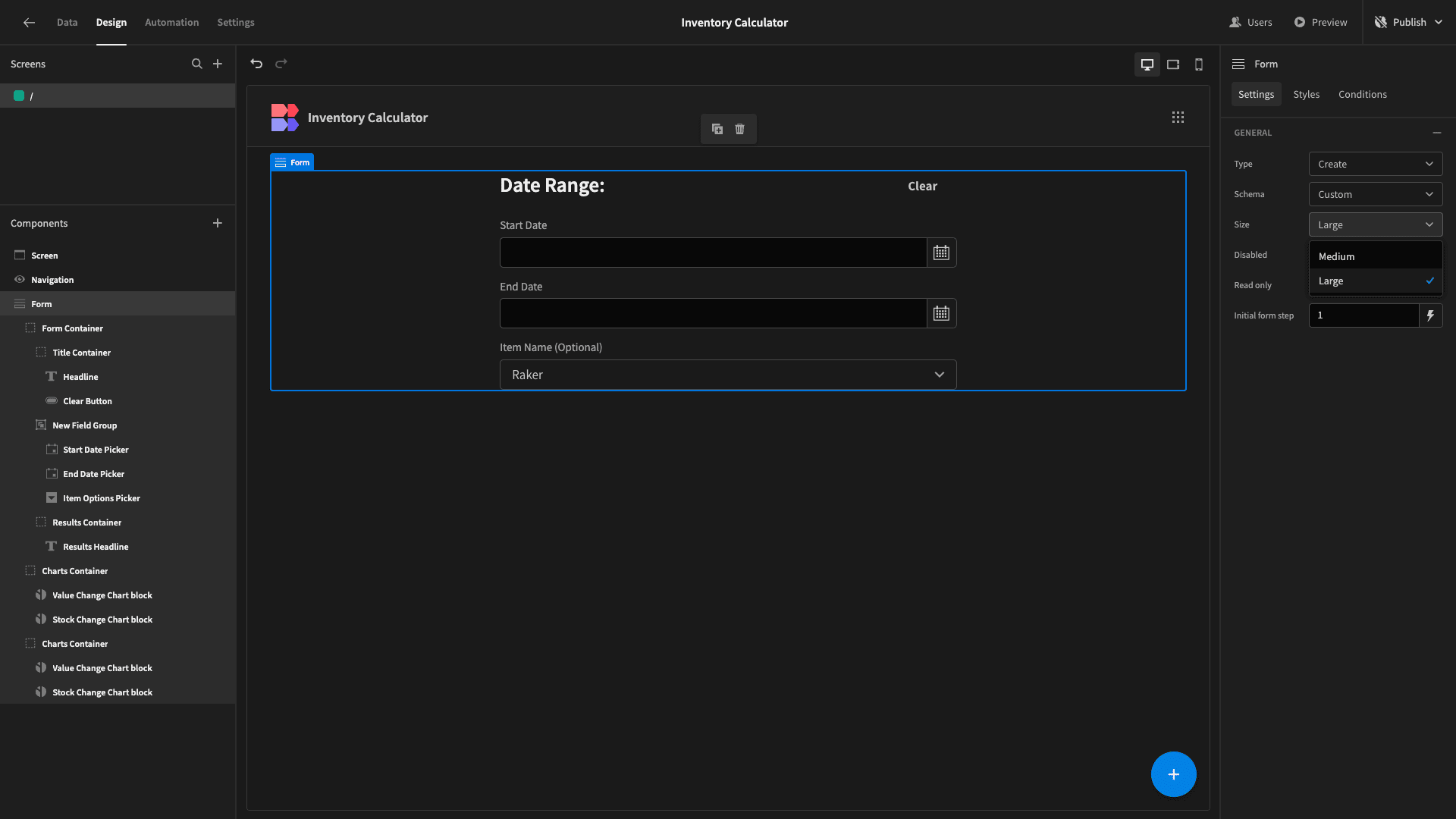
And lastly, under our form component, we’ll set the size to large:

Here’s a reminder of what the finished product looks like:

If you found this tutorial helpful, why not also check out our guide on how to build a supply chain dashboard .